Lesson 10: ROC analysis of neuronal responses

The general purpose of ROC analysis is to provide a measure of the difference between two distributions. For example, Britten et al. (1992) originally used an ROC analysis to determine how well a neuron can 'discriminate' between two stimuli. In this lesson we'll apply an ROC analysis to example spike data measure a neuron's 'neurometric function'.

Contents

The Neurophysiological Data

Britten et al. (J. Neurosci, 1992) measured the spike rates from direction selective neurons in Macaque area MT with the goal of comparing these neuronal responses to the monkey's behavioral data on the same motion coherence task that we developed in the previous lessons.

Their goal was to compare this behavioral data to the MT responses to see how well the results from an individual neuron can predict the behavioral data.

The data set consists of the number of spikes measured in each of 60 trials across five coherence values (.8,1.6,3.2,6.4 and 12.8%) with motion either in the preferred direction or in the direction opposite to the preferred direction of the neuron.

I've generated a fake data set with numbers that are similar to the example neuron they show in their figure 5. We'll load it in now:

clear all
load NeuroData

The file 'NeuroData' contains three parameters:

cList: the list of five coherence values

respPref: of size 5x60 where each row corresponds to a coherence value
and each column corresponds to a trial.  The values are the total
number of spikes for that trial for a stimulus in the preferred
direction.

respNonPref: same thing but for motion in the non-preferred direction.

First, let's look at histograms of the data, plotted like Britten et al.'s figure 5:

figure(1)
clf
for i=1:length(cList)
    subplot(length(cList),1,length(cList)-i+1)
    hist([respPref(i,:);respNonPref(i,:)]',linspace(0,150,40));
    set(gca,'XLim',[0,150]);
    title(sprintf('Coherence %5.1f %%',100*cList(i)),'FontSize',12)
    if i==1
        xlabel('Response (spikes/trial)','FontSize',12);
    end
    set(gca,'FontSize',12);
end

set(gcf,'Position',[220    50   601   680]);

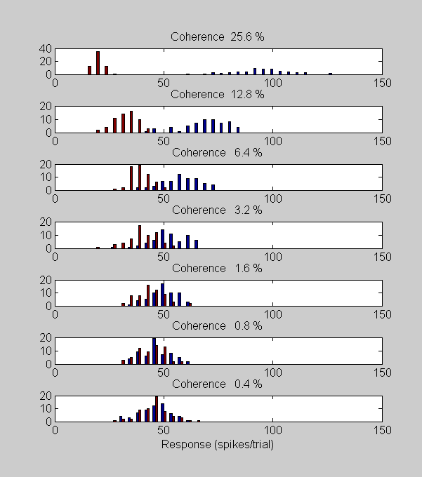
Blue bars in the histograms correspond to responses in the preferred direction and red bars are for the non-preferred direction. Notice how the histograms spread apart as the coherence increases. The neurons are responding more with increased coherence in the preferred direction and are becoming suppressed with increased coherence in the non-preferred direction. This means that, loosely speaking, the neuron more and more able to 'discriminate' between the two stimuli with increasing coherence.

Like humans, the monkey's behavioral performance increased with motion coherence. So at least qualitatively, the neuronal responses are consistent with the behavioral results. But how do we quantify the performance of the neuron? Specifically, for a given motion coherence, how well could you do in the task if all you knew about the stimulus were the responses shown in the histogram above?

The answer can be found with an ROC analysis. We can think of the analysis as an ideal observer performing a 'yes/no' task on samples from the data. Suppose this observer receives a spike count from a stimulus that had, say, 1.6% coherence. The observer must choose a criterion and decide that the stimulus was in the preferred direction if the response exceeds this criterion, otherwise it must have been a non-preferred stimulus. We can calculate how well this observer will do on the task based on the data:

To be specific, let's choose a criterion of 50 spikes/sec:

criterion = 50;

The proportion of 'hits' will be the proportion of times that a preferred stimulus produces a response greater than the criterion:

cNum = 2;  %index into the 0.8% coherence row
nTrials = size(respPref,2);  %number of trials

pHit = sum(respPref(cNum,:)>criterion)/nTrials

% The proportion of false alarms will be the proportion of spike counts
% from the non-preferred data that exceeds the criterion:

pFA = sum(respNonPref(cNum,:)>criterion)/nTrials

pHit =

    0.3333


pFA =

    0.1667

This is the expected performance for this one value of the criterion. To estimate the overall performance, we make this calculation for the whole range of criterion values which will generate an ROC curve. We'll do this for each of the coherence values in a nested loop:

critList = 0:max(respPref(:));   %list of criterion values

pHit = zeros(length(critList),length(cList));
pFA =  zeros(length(critList),length(cList));
for cNum = 1:length(cList)
    for critNum = 1:length(critList)
        criterion = critList(critNum);
        pHit(critNum,cNum) = sum(respPref(cNum,:)>criterion)/nTrials;
        pFA(critNum,cNum) = sum(respNonPref(cNum,:)>criterion)/nTrials;
    end
end

%Let's plot the ROC curve for all coherences:

figure(2)
clf
plot(pFA,pHit,'.-');
legend(num2str(cList'*100),'Location','SouthEast');
set(gca,'XLim',[0,1]);
set(gca,'YLim',[0,1]);
xlabel('p(null>crit)');
ylabel('p(pref>crit)');
set(gca,'XTick',0:.2:1);
set(gca,'YTick',0:.2:1);
hold on
plot([0,1],[0,1],'k-');
axis square

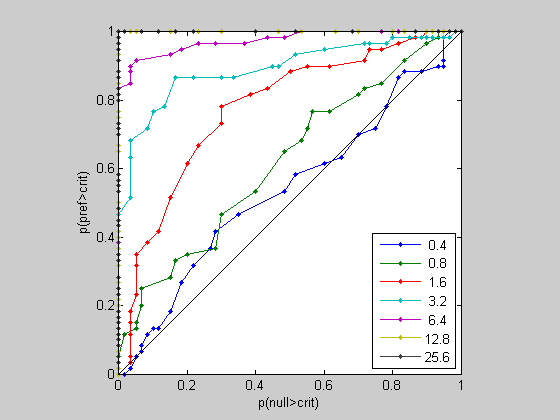
Notice how the ROC curve bows out more and more for higher coherence values. Remember, the area under the curve reflects the difference between the preferred and non-preferred distributions. Let's calculate these values using the 'trapz' function:

for i=1:length(cList)
    AEst(i) = -trapz(pFA(:,i),pHit(:,i));
end

The Neurometric Function

This area under the ROC curve is the best an ideal observer could possibly do given the available data. What we have here is the best possible performance of an observer listening to this neuron as a function of stimulus coherence. This is like a psychometric function, but for the neuron - which is why Britten et al. called this a 'neurometric function'. Let's plot it:

figure(3)
clf
plot(log(100*cList),AEst,'ko-','MarkerFaceColor','b')
set(gca,'XTick',log(100*cList));
set(gca,'YTick',0:0.1:1);
logx2raw
set(gca,'YLim',[.4,1]);
xlabel('Coherence (%)');
ylabel('Proportion correct');

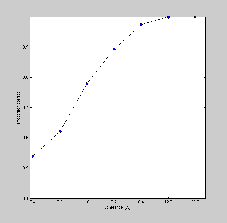
One of the remarkable results from this paper is that the neurometric function from a given neuron matches up well with the monkey's performance on the task - a given neuron is as good at discriminating motion as the monkey!

A simulated 2AFC task

Recall that the area under the curve is the expected performance from a 2AFC task. We can simulate a 2AFC task from our data set by sampling a value from the preferred and non-preferred responses for each trial, and picking off the highest value. This is just like our simulation using signal detection theory where we pulled numbers out of normally distributed signal and noise PDFs.

We need to choose a number of simulated trials. We'll pick a rediculously high number here because we're interested in the performance for the ideal observer, which should effectively have an infinite number of trials:

nSimulatedTrials = 100000;

%Loop through the coherence values
for cNum = 1:length(cList)
    %Draw a list of numbers (with replacement) from each of the two
    %distributions
    internalRespPref = respPref(cNum,ceil(rand(1,nSimulatedTrials)*nTrials));
    internalRespNonPref = respNonPref(cNum,ceil(rand(1,nSimulatedTrials)*nTrials));

    %Get the percent of correct responses by counting up the trials where
    %the draw from the preferred distribution exceeded the non-preferred
    pCorrect(cNum) = sum(internalRespPref>internalRespNonPref)/nSimulatedTrials;
end

hold on
plot(log(100*cList),pCorrect,'ko:','MarkerFaceColor','r');

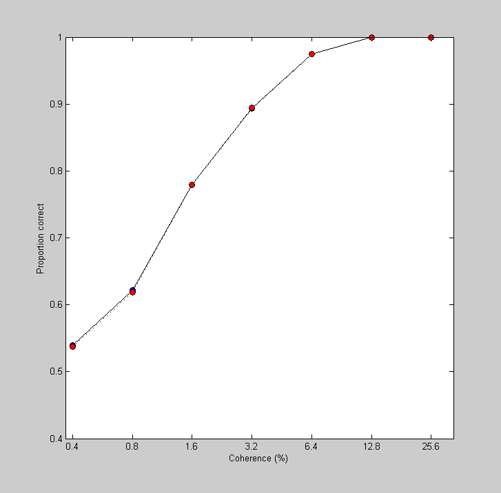
It's a close match. This 2AFC simulation, where we repeatedly draw numbers with replacement from an existing data set, is called a 'bootstrap' method. As you can see, it's a very powerful method. In just a few lines of code we took advantage of the relationship between the area under the ROC and performance on a 2AFC to generate a neurometric function that's essentially identical to the results from the ROC analysis.

Fitting the neurometric function with a Weibull

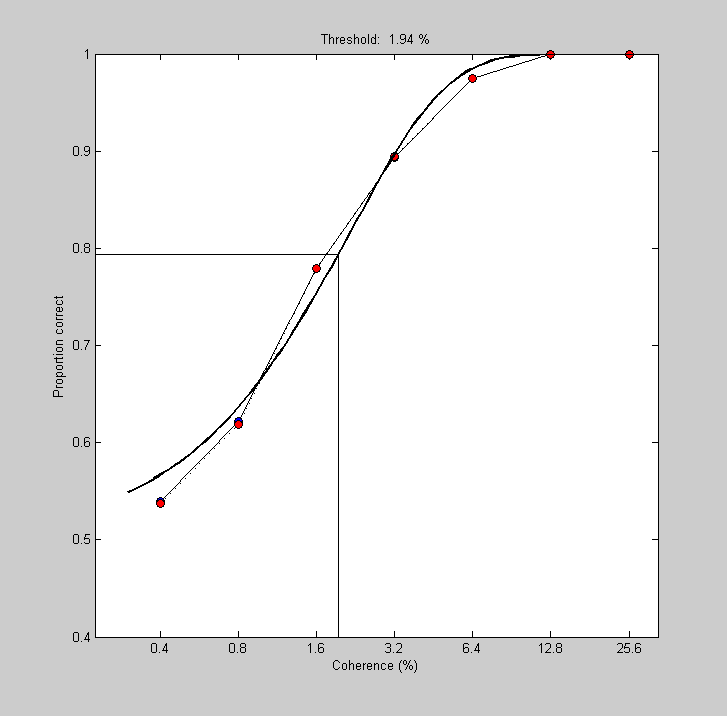
Finally, we can summarize this neuron's ability to detect motion coherence by fitting the neurometric function with a Weibull and estimating the threshold for 80% performance. We've done this enough times now that the following should be self explanatory.

results.intensity = cList;
results.response = pCorrect;

pInit.t = .02;
pInit.b = 2;
freeList = {'b','t'};

[pBest,logLikelihoodBest] = fit('fitPsychometricFunction',pInit,freeList,results,'Weibull');

x = exp(linspace(log(.003),log(.3),101));
y = Weibull(pBest,x);
plot(log(x*100),y,'k-','LineWidth',2);
title(sprintf('Threshold: %5.3g %%',pBest.t*100));
xlim = get(gca,'XLim');
ylim = get(gca,'YLim');
plot([xlim(1),log(pBest.t*100),log(pBest.t*100)],[(1/2)^(1/3),(1/2)^(1/3),ylim(1)],'k-');

Fitting "fitPsychometricFunction" with 2 free parameters.

Published with MATLAB® 7.6