Contents

Lesson 11: 1-D Fourier Transforms

The Fourier Transform is method for representing a 1-dimensional vector (like a time-series) in terms of 'frequencies'. It is typically used to find periodic signals buried in noise, and to design filters that only pass through a specific range of frequencies.

There is an amazing theorem that states that any finitely sampled time-series can be perfectly reconstructed as a sum of a finite number of sinusoids. Moreover, if there are n time-points, then only n/2 sinusoids will be needed.

A sinusoid is defined by three variables, the frequency, the amplitude and the phase. The frequency of the sinusoids needed to reconstruct a time-series is determined by the length of the time series. The first sinusoid will have exactly one cycle, the second will have two cycles, and so on. There's one more sinusoid which has 'zero' frequency, sometimes called the 'dc' (from electrical engineering). This is the mean of the time-series and therefore determines the vertical offset.

Fourier transforms on discretely sampled data are almost always done through an algorithm called the 'Fast Fourier Transform', or FFT. This is a very efficient algorithm (originally developed by Gauss) that is available in all mathematical sofware programs, including Matlab.

Let's start with a trivial example - the Fourier transform of a sinusoid. This is trivial because what we're asking is 'what sinusoids do we need too add together to create a sinusoid'? But this is a good place to start for understanding some of the conventions for the FFT.

First we'll define a 'time' vector on which to calculate our sinusoid. It will be defined by the time-step and the maximum, or ending time:

clear all
dt = .01;
maxt = 1;
t = 0:dt:(maxt-dt);
nt = length(t);  %length of t

Our sinusoid will have 5 cycles, an amplitude of 1 and a phase of zero (with respect to a cosine).

nCycles = 5;
amp = 1;
phase = 0;

This generates a sinusoid of the appropriate number of cycles, amplitude and phase. We'll call it 'y5' because it has 5 cycles. By the way, our phases are defined in degrees, but matlab's 'cos' funtion uses radians. You can convert from degrees to radians by multiplying by pi and dividing by 180.

y5 = amp*cos(2*pi*t*nCycles-pi*phase/180);

This plots the sinusoid

figure(1)
clf
plot(t,y5);
xlabel('Time (s)');
set(gca,'XTick',0:.2:maxt);
set(gca,'YTick',-1:1);
ylabel('Amplitude');
set(gca,'YLim',amp*1.1*[-1,1]);

%'grid' draws dotted lines at the x and y-tick values
grid

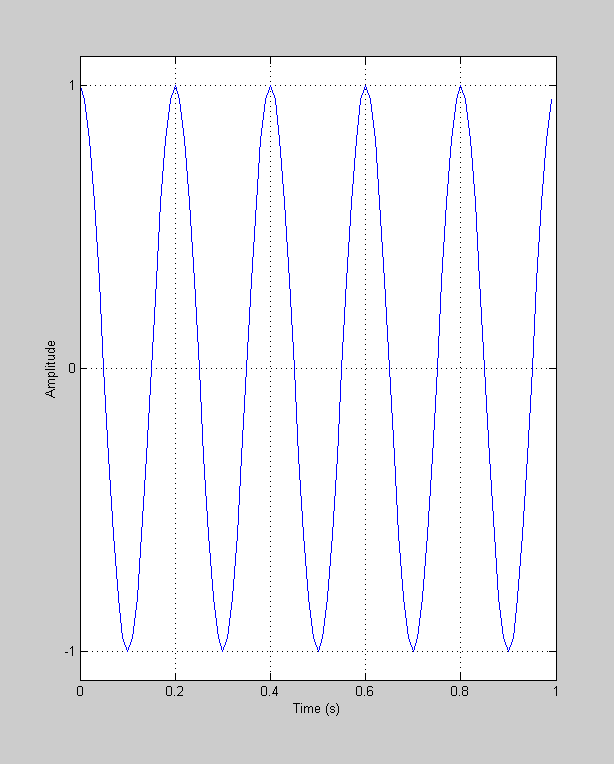
This 5-cycle sinusoid has a frequency of 5 Hz (because the total duration is 1 second). It has an 'amplitude' of 1 (because ranges between -1 and 1) and has a 'phase' of zero (relative to a sine-wave of zero phase).

Matlab's 'fft' function will take the Fourier transform of this vector:

Y5 = fft(y5);

The size of fft(y) is the same as the size y itself. Matlab's 'whos' function is like the 'who' function that lists all your variables, except that 'whos' also tells you its size:

whos y Y

The difference is that 'Y' is of class 'double complex'. What does this mean? Let's take a look at the first few elements of Y:

Y5(1:10)'

ans =

   0.0000          
  -0.0000 - 0.0000i
  -0.0000 + 0.0000i
  -0.0000 + 0.0000i
  -0.0000 + 0.0000i
  50.0000 + 0.0000i
   0.0000 + 0.0000i
   0.0000 - 0.0000i
   0.0000 + 0.0000i
   0.0000 - 0.0000i

Complex numbers

Numbers with the 'i' part are 'complex' numbers. Whoever originally named these numbers 'complex' should be shot (although he's long since dead). Complex numbers aren't that 'complex'. You can really think of them as a shorthand way of representing points on a 2-D plane.

Complex numbers are sums of 'real' and 'imaginary' parts (there's another frightening word: 'imaginary'). Expressed as z = a+ib, 'a' is the real part, 'b' is the imaginary part. In the 2-D plane, the real part is the x-value and the imaginary part is the y-value.

Each of these complex numbers in Y represents the properties of a given sinusoid. The frequency is determined by the position in the list. The first number is the 'dc' value - which is the zero-frequency value, calculated as the mean of y. This is always a real number. The second entry describes sinusoid having exactly one cycle, the third corresponds to two cycles and so on.

Since our sinusoid has 5 cycles, the 'component' in the FFT that we use to reconstruct this should thererfore be in the 6th entry of Y

Y5(6)

ans =

  50.0000 - 0.0000i

This sinusoid of 5 cycles has both an amplitude and phase. Since the corresponding complex number has two parts, you can guess that there is a mapping between the real and imaginary parts of this complex number, and the corresponding amplitude and phase of the sinusoid.

You can plot complex numbers in matlab using the regular 'plot' function. The complex number shows up on a 2-D axis. We'll plot a line between the origin and Y(6) this way:

figure(2)
clf
plot([0,Y5(6)],'ko-','MarkerFaceColor','b');

xlabel('Real component')
ylabel('Imaginary component');
axis equal

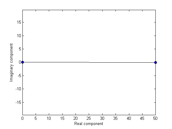
This number has a real component of 50, and an imaginary component of zero. 50? This number is a convention specific to FFT. To convert it to the actual amplitude of the sinusoid component we need to scale it by nt/2. We'll do this now and re-plot (and rescale the axis to include negative numbers).

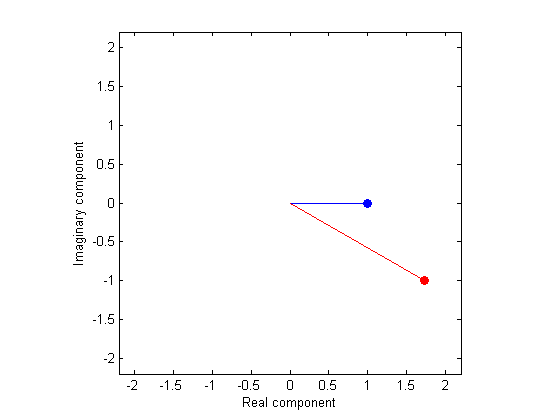
figure(2)
clf
plot([0,2*Y5(6)/nt],'b-');
hold on
h5=plot(2*Y5(6)/nt,'bo','MarkerFaceColor','b');
axis equal

xlabel('Real component')
ylabel('Imaginary component');

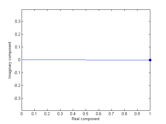
Converting real and imaginary to amplitude and phase

The amplitude is represented by the length of this vector. The phase of our sinusoid (with respect to a cosine) is represented by the angle of the line clockwise from 3 o'clock. You can see from the figure that the amplitude is 1 and the phase is zero.

Let's do this again for a sinusoid having 7 cycles and a different amplitude and phase:

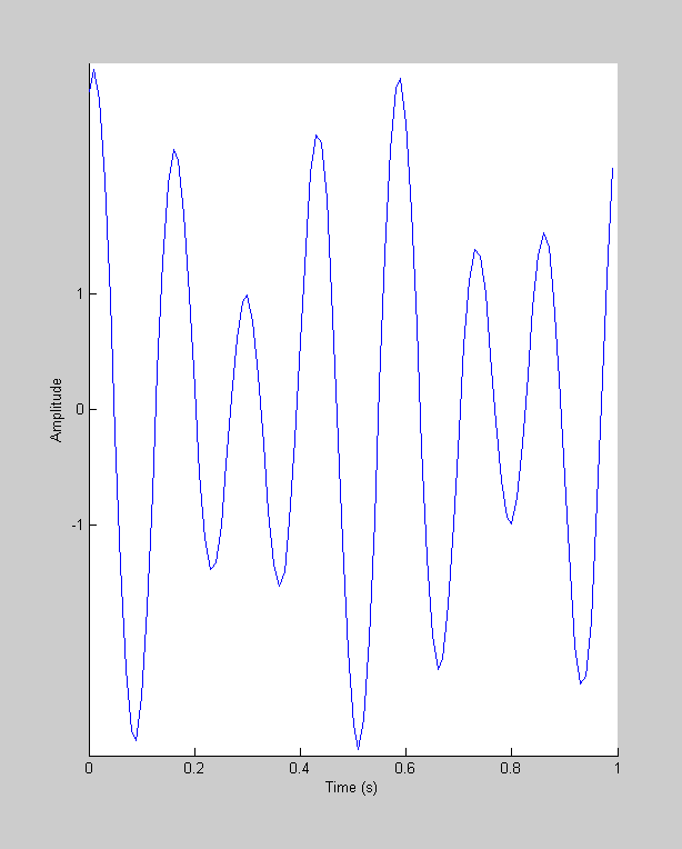
nCycles = 7;
amp = 2;  %around 1.15
phase = 30;  %degrees

y7 = amp*cos(2*pi*t*nCycles-pi*phase/180);

figure(1)
hold on
plot(t,y7,'r-');
xlabel('Time (s)');
set(gca,'XTick',0:.2:maxt);
set(gca,'YTick',-1:1);
ylabel('Amplitude');
set(gca,'YLim',amp*1.1*[-1,1]);
axis square
grid off

Y7 = fft(y7);

The interesting compenent of y7 should be in the eighth entry, right?

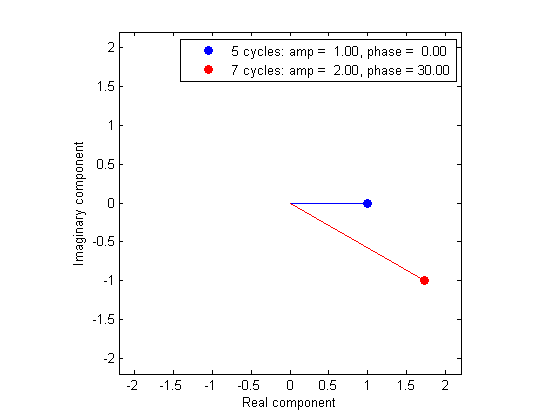
figure(2)
hold on
plot([0,2*Y7(8)/nt],'r-');
h7= plot(2*Y7(8)/nt,'ro','MarkerFaceColor','r');

set(gca,'XLim',1.1*amp*[-1,1]);
set(gca,'YLim',1.1*amp*[-1,1]);

Look how the length of the vector is 2 and the angle is 30 degrees.

To convert a complex number into phase and amplitude, we use matlab's 'amp' and 'phase' functions. The phase of a complex number is the angle in the COUNTERclockwise directon from 3 O'clock. So the convention of the FFT reverses the phase. Again, I dunno why. Taking all this into account, we can reconstruct the amplitudes and phases for our two sinusoides like this:

amp5 = 2*abs(Y5(6))/nt;
phase5 = -180*angle(Y5(6))/pi;

amp7 = 2*abs(Y7(8))/nt;
phase7 = -180*angle(Y7(8))/pi;

txt5=sprintf('5 cycles: amp = %5.2f, phase = %5.2f',amp5,phase5);
txt6=sprintf('7 cycles: amp = %5.2f, phase = %5.2f',amp7,phase7);

legend([h5,h7],{txt5,txt6})

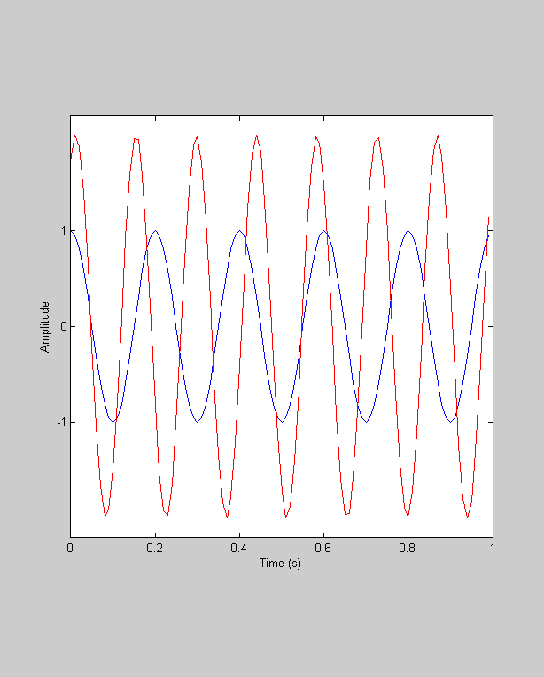
'cosine' and 'sine' components of a sinusoid

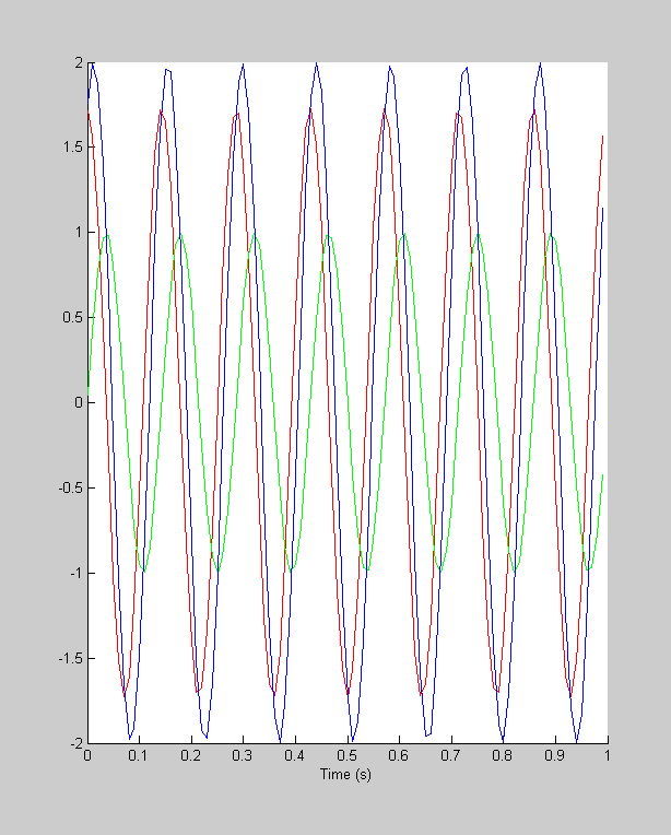
We've shown how to convert a complex number into the corresponding sinusoid's amplitude and phase, but what do the real and imaginary components mean? Another way of representing the two parameters of a sinusoid are by its 'cosine' and 'sine' components, which correspond to the real and imaginary parts of the complex numbers in the FFT. This is based on the trig identity that a sinusoid of any phase and amplitude can be constructed as the sum of a cosine and sine (each with zero phase). We have to flip the sign of the imaginary part as per the convention of the FFT (this is the same as fliping the sign of the phase). The real and imaginary parts of a complex number can be obtained in matlab with 'real' and 'imag'.

realPart = 2*real(Y7(8))/nt;
imagPart = -2*imag(Y7(8))/nt; %note the negative

y7cos = realPart*cos(2*pi*t*7);
y7sin = imagPart*sin(2*pi*t*7);

figure(1)
clf
hold on
plot(t,y7cos,'r-');
plot(t,y7sin,'g-');
plot(t,y7cos+y7sin,'b-');
xlabel('Time (s)');

This plots the original 'y7' sinusoid as black dots to see how it matches up with the reconstructed sinusoid

plot(t,y7,'k.');

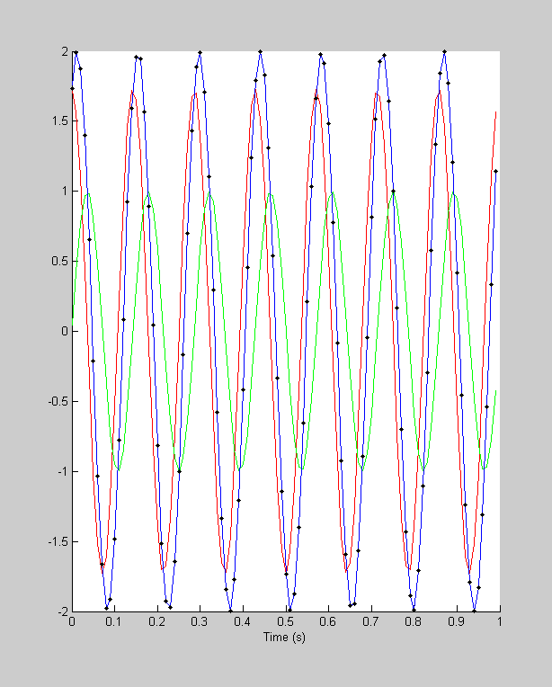
You've now seen how we've reconstructed the sinusoidal components of a simple sine-wave (simple as far as the FFT is concerned).

Now we'll move on to more complicated time-series. The next most complicated thing is a time-series with two sinusoidal components. We can generate this by adding up y5 and y7:

y57 = y5+y7;

figure(1)
clf

hold on
plot(t,y57);
xlabel('Time (s)');
set(gca,'XTick',0:.2:2);
set(gca,'YTick',-1:1);
ylabel('Amplitude');

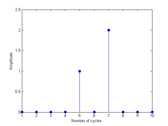
You can guess what happens when we take the fft of this curve:

Y57 = fft(y57);

% We'll plot the amplitudes of the first 10 sinusoids as a 'stem' plot

id = 2:11;  %sinusoids of periods 1 through 10

figure(2)
clf
stem(2*abs(Y57(id))/nt,'fill')

xlabel('Number of cycles')
ylabel('Amplitude');

The Nyquist Limit

What is the highest frequency on the list? If there are n time-steps, then we need n/2 frequencies. The highest frequency is then n/2 cycles per time-series. Think about a sinusoid that has n/2 cycles over n time points. There will be exactly two samples per cycle. Depending on the phase, these samples could either land at the peaks and troughs of the sinusoid, or they could land exactly where the sinusoid crosses zero. It is clear that this is the limit, and going any higher than 2 samples per cycle will start missing crucial properties of the sinusoid. This upper limit of n/2 cycles is called the 'Nyquist Limit'.

Linearity

See how there are only two non-zero amplitudes - the two sinusoids corresponding to 5 and 7 cycles, which is how we built the sinusoid. This illustrates the 'linear' property of the fft: The fft of the sum of two time-series is the same as the sum of the fft of each time series. It also shows a conventional way to represent the results of an fft. By showing only the amplitude we've lost our phase information. Because of this, people often forget to consider the phase of the fft

So far we've seen two conventions of the FFT that we had to deal with to interpret the results of fft: (1) rescaling the amplitude by 2/nt and (2) flipping the sign of the phase (and converting to degrees). There's a third convention that has been hidden so far - it has to do with the length of the output of the fft.

The fft is a 'lossless' transformation, meaning that no information is lost. Because of this (and because the sinusoids are mutually 'orthogonal') if there are nt timepoints in our time-series, then exactly nt numbers are needed to represent the transformation. The output of the fft has nt values in it - but each of these values are complex so they 'contain' two numbers. So the output of the fft has twice as many numbers as the input. What gives?

To see this, we'll make a stem plot of the entire list of amplitudes in Y57:

figure(2)
clf
stem(2*abs(Y57)/nt,'fill')

ylabel('Amplitude');

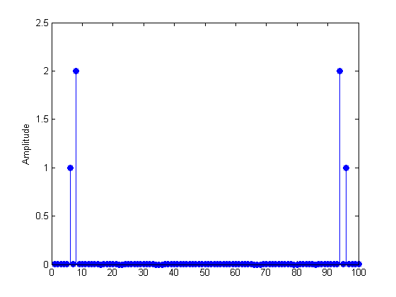
It's mirror symmetric. So each amplitude shows up twice. Here's a closer look at the first and last 7 values in Y57:

Y57(2:8)'
Y57((end-6):end)'

ans =

  -0.0000 + 0.0000i
   0.0000 + 0.0000i
  -0.0000 - 0.0000i
   0.0000 - 0.0000i
  50.0000 - 0.0000i
  -0.0000 + 0.0000i
  86.6025 +50.0000i


ans =

  86.6025 -50.0000i
  -0.0000 - 0.0000i
  50.0000 + 0.0000i
   0.0000 + 0.0000i
  -0.0000 + 0.0000i
   0.0000 - 0.0000i
  -0.0000 - 0.0000i

They're not quite the same - the imaginary parts in the second half are reversed in sign (called the complex conjugate). This means that the phases in the second half are the negative of the first half - and are therefore in proper cosine phase. But otherwise, you can see that the numbers in the second half of the list are redundant.

Why the redundancy? One reason is to deal with complex-valued time-series data. This isn't common in the behavoiral sciences but it does show up in electrical engineering, for example.

It has been a good exersize to walk through the format of the output of the fft because it shows up in computer programs all over the place. But it is clearly cumbersome and confusing because of the complex values, scale factors and redundancy. I've provided a function 'complex2real' that the output of the fft into 'real' values of amplitudes and phases (in degrees). It also provides a vector of corresponding frequencies. We'll use this from now on. Here's an example:

y = t<.5; %a 'step function that's 1 for t<.5
F = fft(y);
Y = complex2real(F,t)  %generates a structure of 'real' amplitudes and phases

Y = 

      dc: 0.5000
      ph: [1x50 double]
     amp: [1x50 double]
    freq: [1x50 double]
      nt: 100

The fields of Y contain the dc and the amplitudes and phases for each frequency. It also provides 'freq' which is a list of corresponding frequencies (in Hz). We can plot y and it's fft like this:

figure(1)
clf
subplot(1,2,1)
plot(t,y);
xlabel('Time (s)');
ylabel('Amplitude');
set(gca,'YLim',[-.05,1.05]);

subplot(1,2,2)
stem(Y.freq,Y.amp,'fill');
set(gca,'XLim',[0,max(Y.freq)]);
xlabel('Frequency (Hz)');
ylabel('Amplitude');

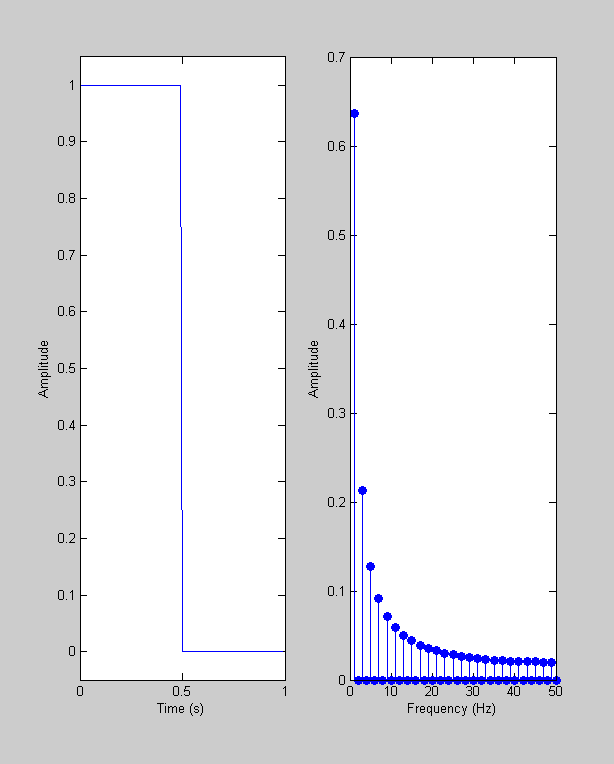
This shows a 'step function' and the corresponding amplitudes of its Fourier Transform. Remember that the amplitudes show what sinusoids are needed to reconstruct the time-series. Notice how every other frequency has an amplitude, and how the amplitudes decreas with increasing frequency. This is because the step function is an 'odd' function, and the odd-numbered sinusoids are also 'odd'. We only need amplitudes from odd sinusoids to create an odd function.

With 'complex2real' it's easy to plot the fft of a range of functions. Since we're doing this a bunch of times, I've provided a function 'plotfft' that draws the time-series and the amplitude spectrum side-by-side in a single figure.

An interesting example is the 'delta' function - zeros everywhere except for one value;

y = zeros(size(t));
y(20) = 1;

plotfft(t,y);

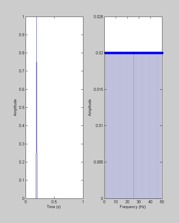
Reconstructing the simplest function you can think of requires a contribution from all frequencies - and all at the same amplitude.

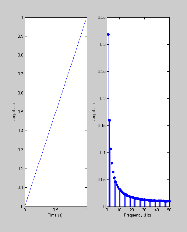
Ramps have an interesting frequency spectrum:

y = t;
plotfft(t,y);

A particularly interesting and common example is the 'Gabor', which is the product of (or 'windowed by') a Gaussian and a sinusoid:

freq = 10; %'carrier' frequency
w = .1;   %'1/e width' of the Gaussian
y = exp(-(t-.5).^2/w^2).*sin(2*pi*freq*t);
plotfft(t,y);

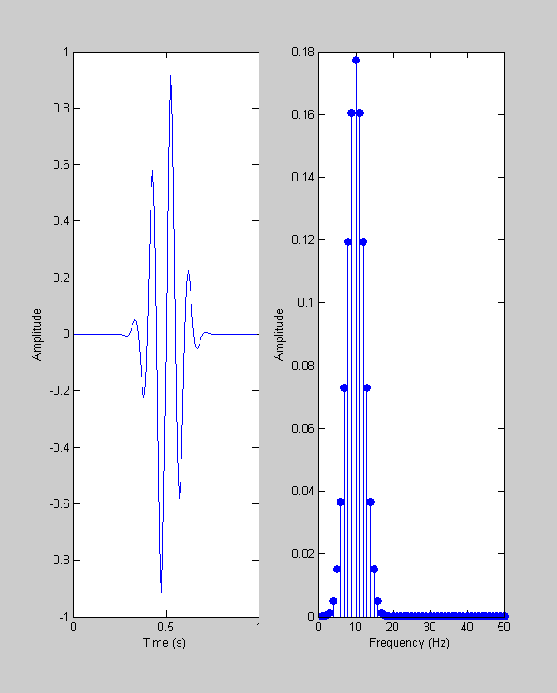
The amplitude plot (sometimes called the 'amplitude spectrum') shows a peak at 10 Hz. This makes sense because a 10Hz sinusoid was used to make the time-series. But since it's not a perfect sinusoid there are other frequencies in there too. They drop off as a Gaussian with the distance from 10Hz. Try playing with the width of the Gaussian. When it's really wide, the time-series is just a sinusoid so the fft will have just one frequency. When it's really narrow, it's like a delta function which has all frequencies. It turns out that the width of the Gaussian used to make the time-series leads to an fft that's a Gaussian with the reciprocal of that width. We'll discuss these 'Gabor' functions more later when we get into linear filters.

Another example is 'white' noise, where every time point is an independent draw from a normal distribution:

y = randn(size(t));
plotfft(t,y);

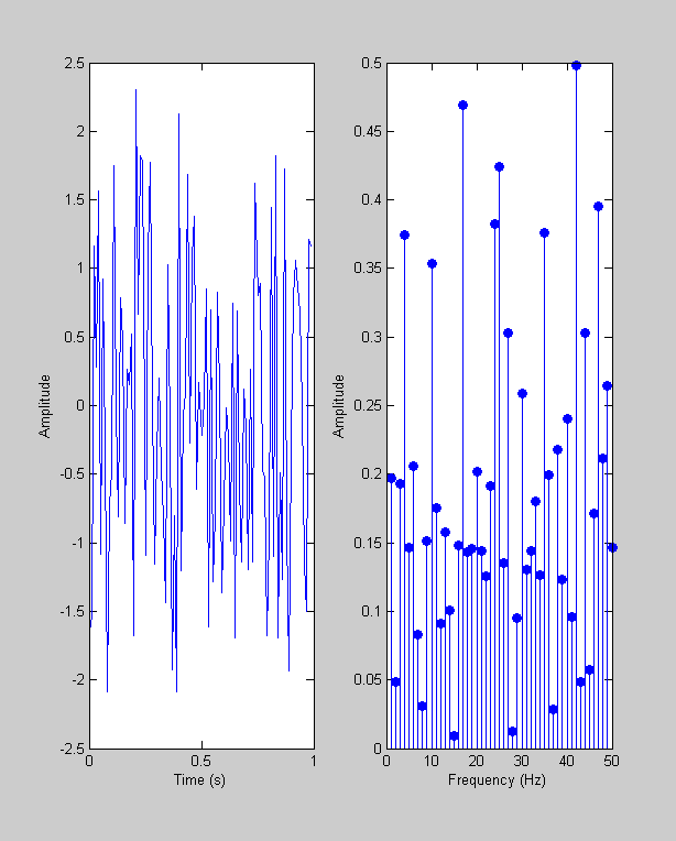
The amplitude spectrum looks like noise too. These amplitudes are also normally distributed with equal probability across all frequencies. White noise contains sinusoids of all frequencies - it's called 'white' presumably because 'white' light contains light of all wavelengths in the spectrum.

Fourier transforms are good at detecting periodic signals buried in noise that is otherwise very difficult to see in the time-series. As an example, we'll add a 12-cycle sinusoid to the random time-series that we just looked at:

nCycles = 12;
y = y+sin(2*pi*nCycles*t);
plotfft(t,y);

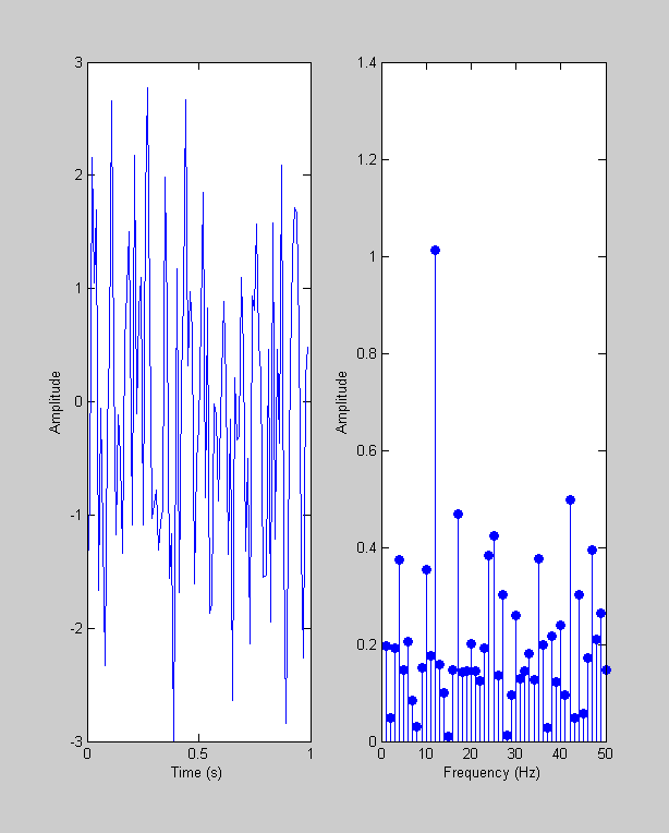
Note the peak in the amplitude spectrum at 12 Hz - not surprising of course, but also notice how difficult it is to see this modulation in the actual time-series.

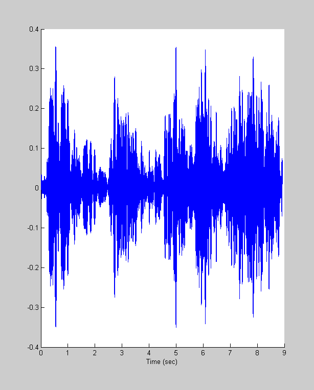
An example: 'handel'

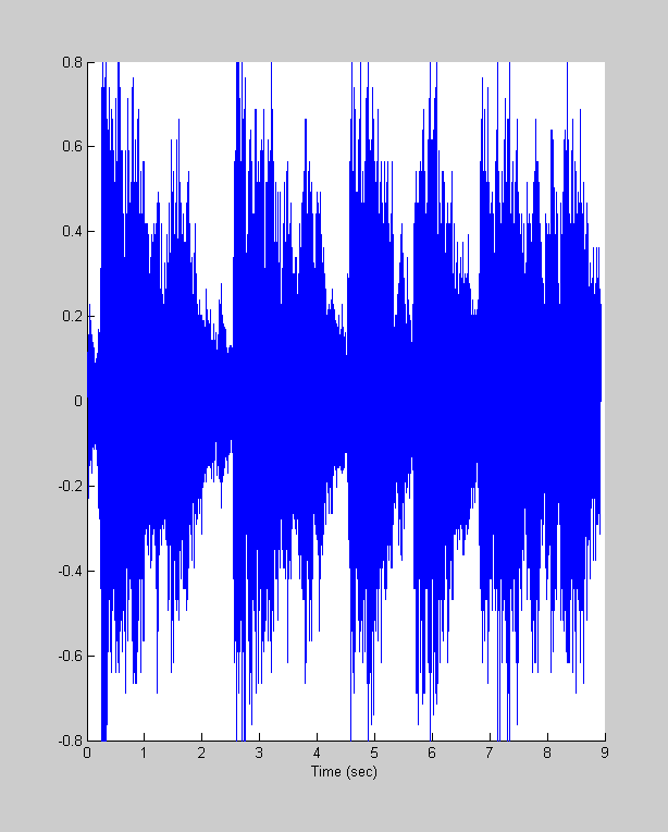
At last we'll apply the fft to something real. Matlab provides some example sounds, including about 8 seconds of Handel's "Hallelujah"

load handel

The file contains two variables, the time-course of the sound, y and the sampling rate, Fs (in Hz). We can create our own time vector from this information:

maxt = length(y)/Fs;
t = linspace(0,maxt,length(y));

% Here's a plot of the time-course of the sound
clf
hold on
plot(t,y);
xlabel('Time (sec)');

Now we'll play the sound, along with a cheesey graphic showing the progress of the sound through the time-course. See if you can figure out how it works. It uses matlab's 'drawnow' feature which updates the graphic upon command. It also uses a handle that's returned from the 'plot' function that allows us to update the x-position of the line. Finally, it takes advantage of matlab's 'sound' function runs the sound in the background so that the animation can take place while the sound is playing.

ylim = get(gca,'YLim');
timeH = plot([0,0],ylim','r-','LineWidth',2);

pause
sound(y,Fs);

tic
while toc<maxt
    set(timeH,'XData',toc*[1,1])
    drawnow
end

delete(timeH);

Let's focus on a particular chunk of the time-sequence between 0.5 and 1. seconds.

tLo = .7;
tHi = .9;

figure(1)
patch([tLo,tHi,tHi,tLo],[ylim(1),ylim(1),ylim(2),ylim(2)],'r','FaceAlpha',.5);

y1 = y(t>tLo & t<tHi);

maxt = length(y1)/Fs;
t1 = t(t>tLo & t<tHi);

%linspace(0,maxt,length(y1));

sound(y1,Fs);

Y1 = complex2real(fft(y1),t1);


clf
subplot(2,1,1)
plot(t1,y1,'k-');
set(gca,'Xlim',[min(t1),max(t1)]);
xlabel('Time (s)');
subplot(2,1,2)
plot(Y1.freq,Y1.amp,'k-');
xlabel('Frequency (Hz)');
ylabel('Amplitude');

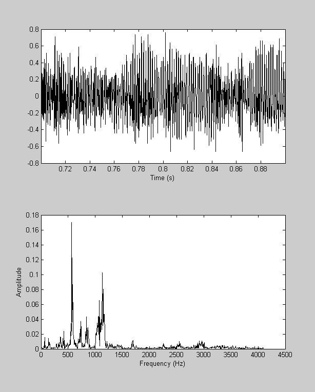
Zoom in on the lower frequencies

set(gca,'XLim',[0,2000]);

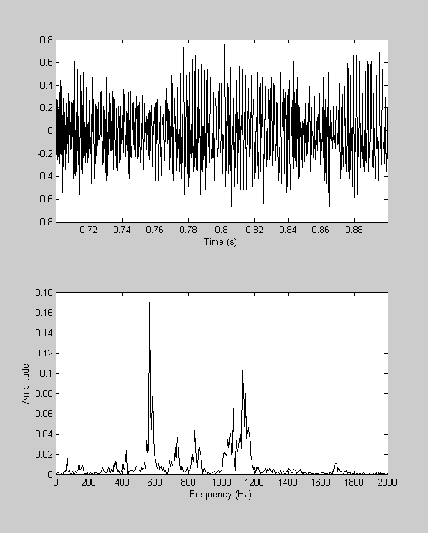
Zoom in again - it looks like there's a peak around 565.

set(gca,'XLim',[530,600]);

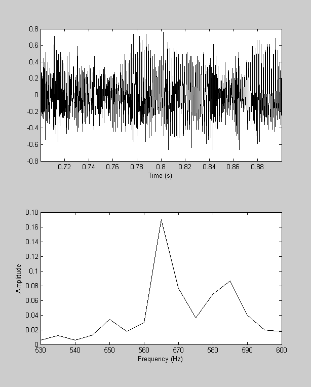
Just for fun, we can generate a sinusoid at 565 Hz and play it - it'll match the fundamental frequency of that first note "Hal" in 'hallelujah'.

y1 = sin(2*pi*565*t1);
sound(y1,Fs);

The Inverse Fourier Transform

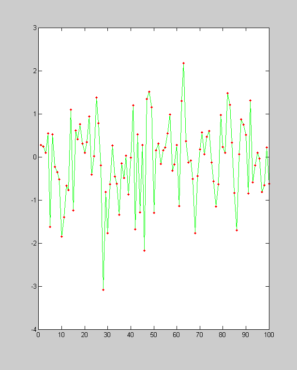
Since the fft is a 'lossless' transform, it is possible to perfectly reconstruct the original time-series from the frequencies and phases we get from the fft. This reconstruction is done through the inverse of the fft, or 'ifft' in Matlab. You can convince yourself that the ifft undoes what the fft does by sending any time-series into the 'frequency domain' and back again. We'll do this with a random time-series

yrand = randn(1,100);
F = fft(yrand);
yrecon = ifft(F);


clf
plot(yrand,'g-');
hold on
plot(yrecon,'r.','MarkerFaceColor','r');

Filtering a time-series using ifft.

Being able to go back and forth into the frequency domain is very useful for filtering. For example, in the 'hallelujah' time-series, we alter the time-series so that it contains only a subset of the original frequencies by modifying the amplitudes after taking the fft:

Y = complex2real(fft(y),t);

% Range of frequencies to keep
fLo = 545;
fHi = 575;

% Set frequencies outside the range to zero
Y.amp(Y.freq>fHi | Y.freq<fLo) = 0;

% Reconstruct the time series
F = real2complex(Y);
yrecon = ifft(F);

clf
hold on
plot(t,yrecon);
xlabel('Time (sec)');

ylim = get(gca,'YLim');
timeH = plot([0,0],ylim','r-','LineWidth',2);

pause
sound(yrecon,Fs);

tic
while toc<maxt
    set(timeH,'XData',toc*[1,1])
    drawnow
end

delete(timeH);

We've just made our first filter! A filter like this that only allows through a middle range of frequencies is called 'band-pass', and our specific example that has a hard cut-off at the low and high range is called a 'notch' filter.

A more common way to make a band-pass filter is to attenuate the frequencies with a smooth Gaussian function. Let's apply a filter with a Gaussian 'envelope' to the response to the delta function:

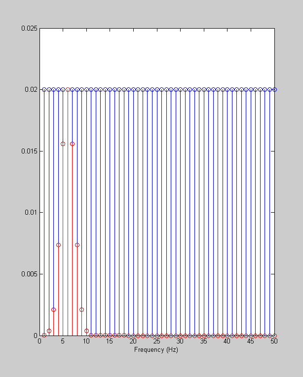
% Re-create the time vector 't'
dt = .01;
maxt = 1;
t = 0:dt:(maxt-dt);
nt = length(t);  %length of t

% Delta function at time point 50
y = zeros(size(t));
y(50) = 1;

% FFT
Y = complex2real(fft(y),t);

figure(1)
clf
stem(Y.freq,Y.amp);
xlabel('Frequency (Hz)');

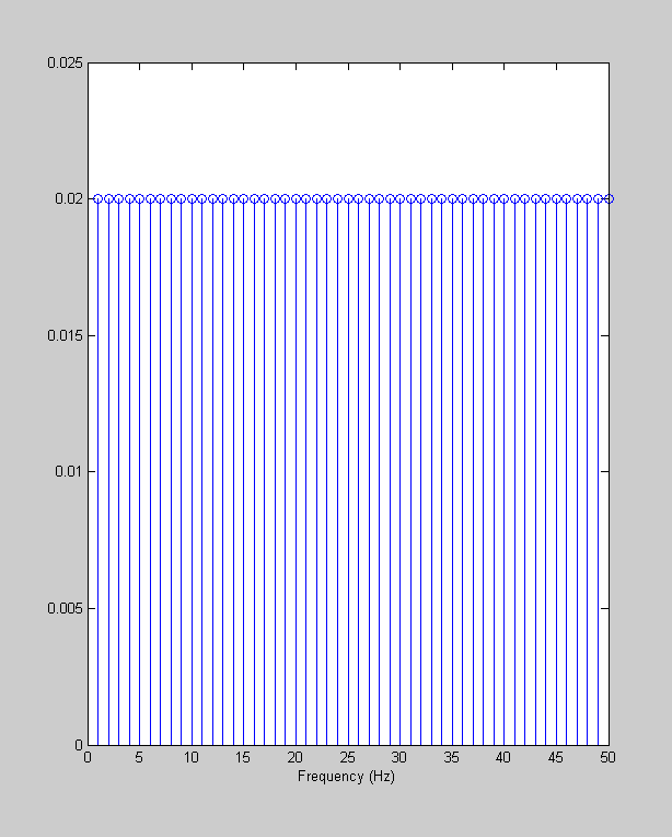
The amplitude spectrum is flat, remember? Now we'll multiply this flat amplitude spectrum by a Gaussian

gCenter = 6; %Hz
gWidth = 2; %Hz
Gauss = exp(-(Y.freq-gCenter).^2/gWidth^2);
Y.amp = Y.amp.*Gauss;
hold on
stem(Y.freq,Y.amp,'r');

Then we'll take the inverse Fourier Transform:

yrecon = real(ifft(real2complex(Y)));
clf
plotfft(t,yrecon);

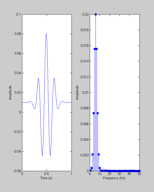
This looks familiar, it's a Gabor! What have we done here? We took a delta function, sent it into 'frequency space', attenuated the frequences with a Gaussian centered at 6 Hz, and sent it back into the 'time-domain' with the inverse fft.

These steps show what happens when we send the delta function through a band-pass filter. The low and high frequences are removed, leaving just the intermediate frequencies, which is exactly how to think about a Gabor: it 'contains' only a limited range of frequencies within a Gaussian envelope.

This response to a delta function is called an 'impulse-response function'. (Technically, a real 'impulse' has infinitely small width and infinite height with area equal to one, but with discrete sampling this is the same idea).

We'll have much more discussion about the impulse response function in the next lesson.

Generating our own spectrograph

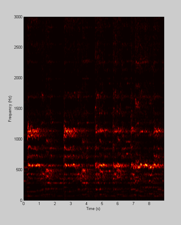
As a final exersize, we'll use the fft to create a 'spectrograph' of the 'handel' time-series. A spectrograph provides the frequency spectrum of a time series as a function of time. One way to get the frequency spectrum at a point in time is to window the time-series around this point with a Gaussian before taking the fft:

load handel

% Vocal sweep
%[y,Fs]=wavread('sweep.wav');


maxt = length(y)/Fs;
t = linspace(0,maxt,length(y));

% Number of time-steps
nSteps = 501;
% Center of each time-step
tCenter = linspace(0,max(t),nSteps);
% Width of Gaussian for windowing:
gaussWidth = .02;  %seconds

% Zero out the 'amp' matrix
nAmps = ceil(length(t)/2);
amp = zeros(length(tCenter),nAmps);

% Loop through the time steps, windowing y and calculating the fft
for i=1:length(tCenter)
    Gauss = exp(-(t-tCenter(i)).^2/gaussWidth.^2)';
    newy = y.*Gauss;
    Y = complex2real(fft(newy),t);
    amp(i,:) = Y.amp;
end

Show the spectrograph as an image using 'imagesc'

figure(1)
clf
imagesc(tCenter,Y.freq,amp');
colormap(hot);
xlabel('Time (s)')
ylabel('Frequency (Hz)');
set(gca,'YDir','normal');
set(gca,'YLim',[0,3000]);

cmap = hot(64);
cmap = cmap.^1;
colormap(cmap);

play the sound, along with the cheesey graphic.

hold on
ylim = get(gca,'YLim');
timeH = plot([0,0],ylim','g-','LineWidth',2);

pause
sound(y,Fs);

tic
while toc<maxt
    set(timeH,'XData',toc*[1,1])
    drawnow
end

delete(timeH);

Exercises

Published with MATLAB® 7.6