Lesson_12 Linear filters for 1-D time-series

A 1-D 'filter' is a function that takes in a 1-D vector, like a time-series and returns another vector of the same size. Filtering shows up all over the behavioral sciences, from models of physiology including neuronal responses and hemodynamic responses, to methods for analyzing and viewing time-series data.

Typical filters are low-pass and band-pass filters that attenuate specific ranges of the frequency spectrum. We built our first filter in the last lesson by specifying which frequencies we wanted to modify using the fft and the ifft. In this lesson we'll focus on the time-domain by developing a simple leaky integrator filter and show that it satisfies the properties of superposition and scaling that make it a linear filter.

Contents

The Leaky Integrator

A 'leaky integrator' possibly the simplest filter we can build, but it forms the basis of a wide range of physiologically plausible models of neuronal membrane potentials (such as the Hodgkin-Huxley model), hemodynamic responses (as measured with fMRI), and both neuronal and behavioral models of adaptation, such as light and contrast adaptation.

A physical example of a 'leaky integrator' is a bucket of water with a hole in the bottom. The rate that the water flows out is proportional to the depth of water in the bucket (because the pressure at the hole is proportional to the volume of water). If we let 'y(t)' be the volume of water at any time t, then our bucket can be described by a simple differential equation:

Where 'k' is the constant of proportionality. A large 'k' corresponds to a small hole where the water flows out slowly. You might know the closed-form solution to this differential equation, but hold on - we'll get to that later.

We need to add water to the bucket. Let s(t) be the flow of water into the bucket, so s(t) adds directly to the rate of change of y:

A physiological example of a leaky integrator is if 'y' is the membrane potential of a neuron where the voltage leaks out at a rate in proportion to the voltage difference (potential) and 's' is the current flowing into the neuron. This is the basis of a whole class of models for mebrane potentials, including the famous Hodgkin-Huxley model.

We can easily simulate this leaky integrator in discrete steps of time by changing the value of 'y' on each step according to the equation above:

clear all

% Generate a time-vector
dt = .001;  %step size (seconds)
maxt = 5;  %ending time (secons)
t = 0:dt:(maxt-dt);
nt = length(t);  %length of t

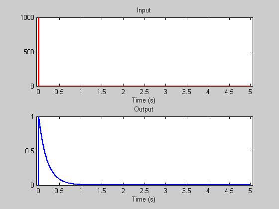
%As our first example, we'll let k=inf, so there's no hole in the bucket
%(or the hole is infinitely small).
k = inf;

% Define 's' to be one for the first second.
s  = zeros(size(t));
s(t<=1) =1 ;

Here's the loop.

y =zeros(size(t));
for i=1:(nt-1)
    dy = s(i)-y(i)/k;
    y(i+1)=y(i)+dy*dt;
end

figure(1)
clf
plotResp(t,s,y);

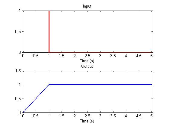
Next we'll add the hole in the bucket by setting 'k' to 1. I've written a function 'leakyIntegrator' that does the loop above since we'll be using this a bunch of times in this lesson.

k=1;
y = leakyIntegrator(s,k,t);
clf
plotResp(t,s,y);

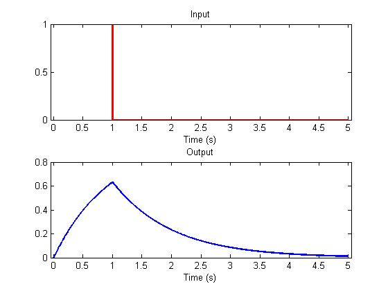
See how the bucket starts filling up more slowly, and how the water drains out when the flow stops. Try this again with a bigger hole by letting k = 1/5 = .2, for example:

k=.2;
y = leakyIntegrator(s,k,t);
plotResp(t,s,y);

This time the water reached an asymptotic level. This is because the flow rate out the bottom eventually reached the rate of flow into the bucket. With k=.2, can you figure out why the asymptotic level is 0.2? Notice also how the water drains out more quickly. The size of the hole, 'k', is called the 'time-constant' of this leaky integrator.

Responses to short impules

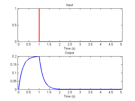
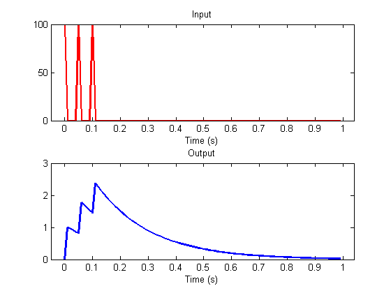
Our previous example had water flowing into the bucket at 1 gallon/second for one second. What happens when we splash in that gallon of water in a much shorter period of time, say within 1/10 of a second.

figure(1)
clf
k = 1/5;
s = zeros(size(t));
dur = .01;
s(t<dur) = 1/dur;
y = leakyIntegrator(s,k,t);
plotResp(t,s,y);
subplot(2,1,1)


set(gca,'YLim',[0,1]);

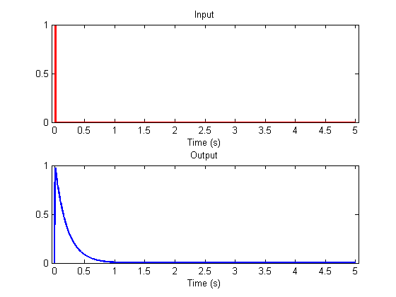
Here's the same amount of water splashed in 1/100 of a second.

figure(2)
clf

k = 1/5;
s = zeros(size(t));
dur = .001;
s(t<dur) = 1/dur;
y = leakyIntegrator(s,k,t);
plotResp(t,s,y);

set(gca,'YLim',[0,1]);

Compare these two responses - they're nearly identical. This is because for short durations compared to the time-constant, the leaky integrator doesn't leak significantly during the input, so the inputs are effectively the same.

How long can you let the stimulus get before it starts significantly affecting the shape of the response? How does this depend on the time-constant of the leaky integrator?

This behavior is an explanation for "Bloch's Law", the phenomenon that brief flashes of light are equally detectable as long as they are very brief, and contain the same amount of light. Indeed, the temporal properties of the early stages of the visual system are typically modeled as a leaky integrator.

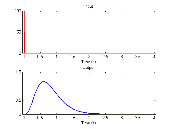
This response to a brief '1-gallon' (or 1 unit) stimulus is called the 'impulse response' and has a special meaning which we'll get to soon.

Scaling

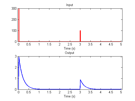
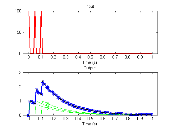
It should be clear by the way the stimulus feeds into the response that doubling the response doubles the peak of the response. Since the recovery falls of in proprtional to the current value, you can convince yourself that the whole impulse-response scales with the size of the input. Here's an example of the response to two brief pulses of different sizes separated in time. You'll see that the shape of the two responses are identical - they only vary by a scale-factor. This is naturally called 'scaling'. Mathematically, if L(s(t)) is the response of the system to a stimulus s(t), then L(ks(t)) = kL(s(t)).

dt = .001;  %step size (seconds)
maxt = 5;  %ending time (secons)
t = 0:dt:(maxt-dt);

dur = .01;
amp = 3/dur;
s = zeros(size(t));
s(t<dur) = amp;

s(t>=3 & t<3+dur) = 1/dur;

y = leakyIntegrator(s,k,t);
figure(1)
clf
plotResp(t,s,y);

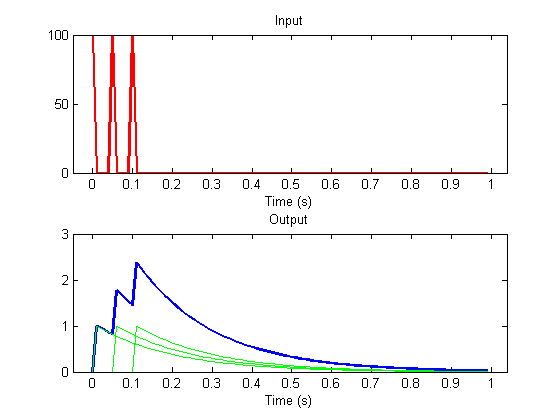
Superposition

In the last example, the second stimulus (splash of water) occurred long after the response to the first stimulus was over. What happens when the second stimulus happens sooner?

dt = .001;  %step size (seconds)
maxt = 2;  %ending time (secons)
t = 0:dt:(maxt-dt);

dur = .01;
t1 = 0;  %time of first stimulus onset
s1 = zeros(size(t));
s1(t>=t1 & t<t1+dur) = 1/dur;

y1 = leakyIntegrator(s1,k,t);  %response to first stimulus


t2 = .1;  %time of second stimlus onset
s2 = zeros(size(t));
s2(t>=t2 & t<t2+dur) = 1/dur;

y2 = leakyIntegrator(s2,k,t);

%Response to the sum of the stimuli:
y12 = leakyIntegrator(s1+s2,k,t);

%Plot the response to the sum of the two stimuli:
figure(1)
clf
plotResp(t,s1+s2,y12);

% Plot the response to each of the stimuli alone:

hold on
plot(t,y1,'g-');
plot(t,y2,'g-');

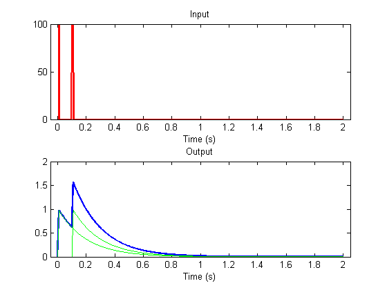
You can see that the response to the sum (y12) is equal to the sum of the response to the individual stimuli (y1 + y2). That is:

L(s1+s2) = L(s1)+L(s2)

This property is called 'superposition'. By the way, we're also assuming that the time-constant is fixed so that the shape of the response to a stimulus doesn't vary with when it occurs. This property is called 'shift' invariance.

A system that has both the properties of scaling and superposition is called a 'linear system', and one with shift invariance is (naturally) called a 'shift-invariant linear system'.

Analytical solution for the leaky integrator

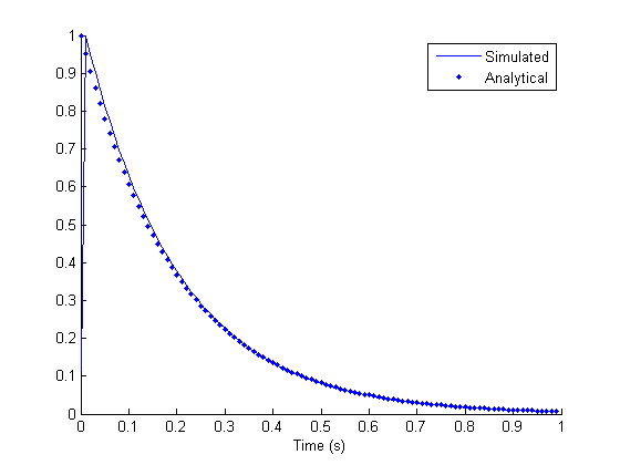
The differental equation that describes the leaky integrator is very easy to solve analyitically. If $$\frac{dy}{dt} = -\frac{y}{k}$$ Then $$\ydy = -\frac{1}{k} dt $$ Integrating both sides: $$\log(y) = -\frac{t}{k} + C $$ Exponentiating: $$ y = e^{-\frac{t}{k}+C} $$ To calculate the impulse response, we let y(0) = 1, which makes C=0. $$ y = e^{-\frac{t}{k}} $$

Let's compare the simulated to the analytical impulse response:

dt = .01;  %step size (seconds)
maxt = 1;  %ending time (secons)
t = 0:dt:(maxt-dt);
nt = length(t);  %length of t

% Calculate the impulse response
s = zeros(size(t));
s(1) = 1/dt;

h = leakyIntegrator(s,k,t);
nht = nt;

hh = exp(-t(1:nht)/k);

clf
hold on
plot(t(1:nht),h,'b-');
plot(t(1:nht),hh,'b.');
legend({'Simulated','Analytical'});
xlabel('Time (s)');

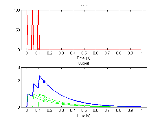
Convolution

The properties of scaling and superposition have a significant consequence - if we think of any complicated input as a sequence of scaled impulses, then the output of the system to this input can be predicted by a sum of shifted and scaled impulse response functions. Here's an example where the input has three impulses at time-points 1, 6 and 11:

t1 = 1;
t2 = 6;
t3 = 11;
s = zeros(size(t));
s([t1,t2,t3]) = 1/dt;

y = leakyIntegrator(s,k,t);
clf
plotResp(t,s,y);

The response at time point, say 16, is predicted by the sum of the response to the three inputs. Each of these three inputs produces the same shaped impulse-response, so the response at time 16 is the sum of the impulse response function evaluated at three points in time.

Plot the response to the three impulses:

subplot(2,1,2);
hold on
for i=1:nht;
    plot(t(i:min(nt,i+nht-1)),s(i)*h(1:nht-i+1)*dt,'g-')
end

The response to the three inputs at time point 16 is the impulse response function evaluated at the time since the input occured:

id =16;

plot(t(id),h(id-t1+1),'go');
plot(t(id),h(id-t2+1),'go');
plot(t(id),h(id-t3+1),'go');

Superposition means that the response to the system is the sum of these three values:

r = h(id-t1+1)+h(id-t2+1)+h(id-t3+1);
plot(t(id),r,'bo');

For any stimulus, the response at time-point 16 is going to be the sum of shifted, scaled versions of the impulse response function. This loop will give us the same number as the calculation above:

rr= 0;
for i= max(1,id-nht):id
    rr =rr + s(i)*h(id-i+1)*dt;
end

plot(t(id),r,'bo','MarkerFaceColor','b');

The response at all time-points can be calculated as above by looping through time:

rr = zeros(size(t));
for j=1:nt
    for i= max(1,j-nht+1):j
        rr(j) =rr(j) + s(i)*h(j-i+1)*dt;
    end
end

h3=plot(t,rr,'k.');

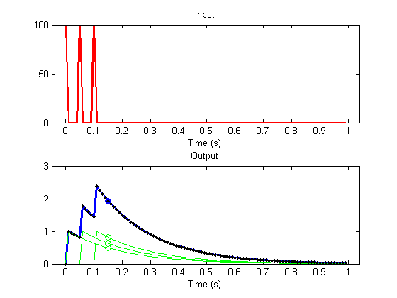
This operation is called 'convolution', and can be implemented by Matlab's function 'conv'. This function takes in two vectors of length m and n and returns a vector of length m+n-1. If the first vector is the stimulus and the second is the impulse response, then you'd think that the output would have length m. It's longer because the function pads the inputs with zeros so that we get the entire response to the very last input. We'll truncate the output to the length of the input:

rconv = conv(s,h)*dt;
rconv = rconv(1:nt);

plot(t,rconv,'bs');

Response to arbitrary stimulus

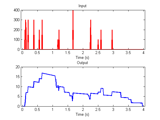
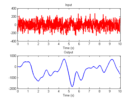
With convolution and the analytical solution to the leaky integrator, we can predict the response to of the system to any input, like a random series of scaled impulses:

dt = .01;  %step size (seconds)
maxt = 4;  %ending time (secons)
t = 0:dt:(maxt-dt);
nt = length(t);  %length of t

k = 1/5;
%Use the analytical form with convolution
h = exp(-k*t(1:nht));

% Here's an input
s = floor(rand(size(t))+.05).*round(rand(size(t))*5)/dt;
s(t>maxt-1) = 0;


y = conv(s,h)*dt;
y = y(1:nt);

figure(1)
clf
plotResp(t,s,y);

Cascades of leaky integrators

It is common to model sensory systems with a 'cascade' of leaky integrators, where the output of one integrator feeds into the input of the next one. The response to an impulse can be simulated in the following for-loop.

s = zeros(size(t));
s(1) =1/dt;
s0 = s;
nCascades = 4;
y = s;
for j=1:nCascades
    y =  leakyIntegrator(y,k,t);
    y = y/k;
end

clf
plotResp(t,s,y);

The impulse response function for a cascade of leaky integrators.

maxt = 10;
t = 0:dt:(maxt-dt);
nt= length(t);

k = 1/5;
h = gamma(nCascades,k,t);
subplot(2,1,2);
hold on
plot(t,h,'b.');

Here's the response of a cascade of leaky integrators to a white noise stimulus:

s = randn(size(t))/dt;

y = conv(s,h);
y=y(1:nt);

clf
plotResp(t,s,y);

See how smooth the output is? If you think about how convolution acts, the response at each time point is the sum of the previous inputs weighted by the impulse-response function going back in time. The impulse response function of the cascade of leaky integrators (the gamma function) is a smooth bump, so the response at any given time is a weighted average of the previous inputs. This effectively smooths out the bumps in the input. Does this sound familar? What do you think this does to the input in terms of frequencies?

Response to sinusoids

Following up on this smoothing observation, we'll look at output of our cascade of leaky integrators to sinusoids of different frequencies.

freq = .4; %Hz
s = sin(2*pi*freq*t);
y =  conv(s,h)*dt;
y = y(1:nt);

clf
plotResp(t,s,y);

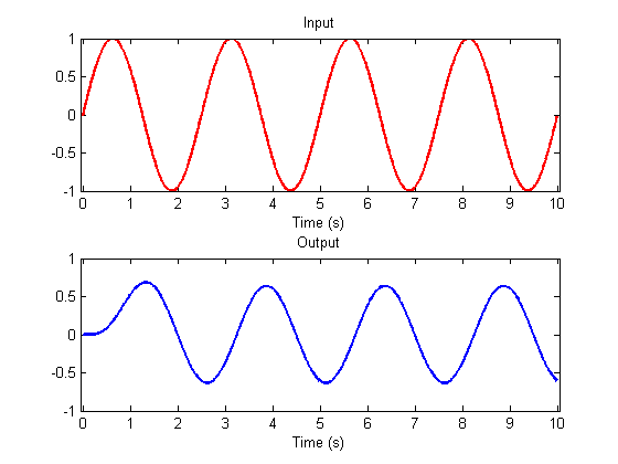
After the inital wobble, the response to a sinusoid is another sinusoid of the same frequency. Only the amplitude and phase has changed. Try a higher frequency:

freq = 2; %Hz
s = sin(2*pi*freq*t);
y =  conv(s,h)*dt;
y = y(1:nt);

clf
plotResp(t,s,y);

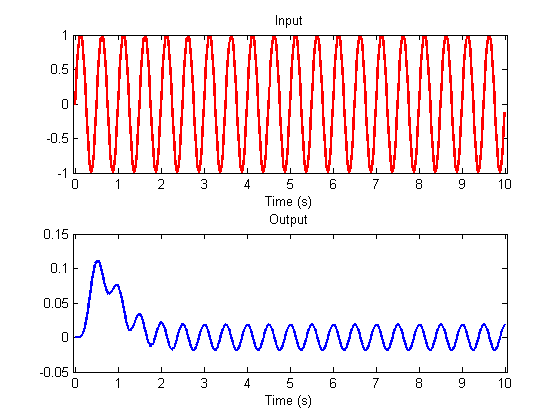
This illustrates a unique property of shift-invariant linear systems: The response to any sinusoid is a sinusoid of the same frequency, scaled in amplitude and delayed in phase (The wobbly part in the beginning is because at the beginning, the input into the filter isn't a complete sinusoid until time has reached the duration of the impulse response).

This only works for sinusoids - other functions (like square waves or whatever) will change shape after being passed through the filter.

Let's calculate the amplitude of the output sinusoid for different frequencies to see how the filter attenuates higher and higher frequencies:

nCycles = 1:20;
amp = zeros(size(nCycles));
for i=1:length(nCycles)
    s = sin(2*pi*nCycles(i)*t/maxt);
    y =  conv(s,h)*dt;
    y = y(1:nt);
    amp(i) = (max(y(t>3))-min(y(t>3)))/2;
end

clf
plot(nCycles,amp,'bo-','MarkerFaceColor','w');
xlabel('Frequency of input (cycles)');
ylabel('Amplitude of output');

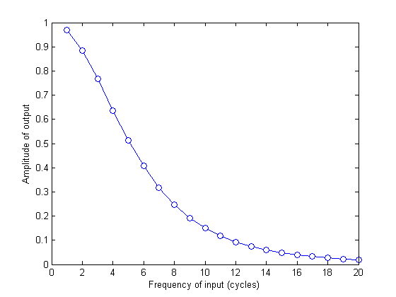
This is attenuation of higher frequencies should follow our intuition of how the high frequencies are taken out of the white noise input. It should also remind you of the 'low-pass' filter that we build in the last lesson using the Fourier transform. In fact, we can learn something interesting by taking the Fourier transform of the impulse response function.

%h = sin(2*pi*4*t/maxt);

H = fft(h);
Hamp = abs(H(nCycles+1))*dt;

hold on
plot(nCycles,Hamp,'b.')

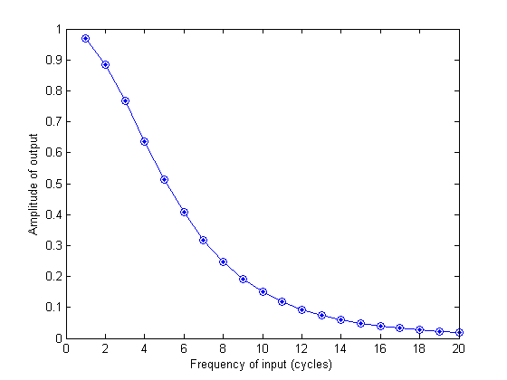
The way a linear filter attenuates a sinusoid matches the amplitudes of the fft of the filter's impulse response function. What's the significance of this?

We have now shown that:

(1) Any time-series can be represented as a sum of scaled sinsoids (2) A linear system only scales and shifts sinusoids (3) The response to the sum of inputs is equal to the sum of the responses (4) The fft of the impulse response determins how the filter scales the sinusoids.

Together, this means that there are two ways to calculate the response to a linear system: (1) convolving with the impulse response function and (2) multiplying the fft of the input with the fft of the impulse response function. Convolution in the time domain equals point-wise multiplication in the frequency domain.

This will make more sense with an example. Remember the band-pass filter we made in the last lesson? The following will do it again.

% Re-create the time vector 't'
dt = .01;
maxt = 1;
t = 0:dt:(maxt-dt);
nt = length(t);  %length of t

% Delta function at time point 50
y = zeros(size(t));
y(50) = 1;

% Take the FFT
Y = complex2real(fft(y),t);

% Attenuate the amplitudes with a Gaussian
gCenter = 6; %Hz
gWidth = 2; %Hz
Gauss = exp(-(Y.freq-gCenter).^2/gWidth^2);
Y.amp = Y.amp.*Gauss;

% Take the inverse Fourier Transform:
yrecon = real(ifft(real2complex(Y)));
clf
plotfft(t,yrecon);

Warning: Could not find an exact (case-sensitive) match for 'plotfft'.
C:\Documents and Settings\Geoff Boynton\My
Documents\courses\Matlab_2_S09\matlab\toolbox\plotFFT.m is a case-insensitive match and
will be used instead.
You can improve the performance of your code by using exact
name matches and we therefore recommend that you update your
usage accordingly. Alternatively, you can disable this warning using
warning('off','MATLAB:dispatcher:InexactCaseMatch').
This warning will become an error in future releases.

The impulse response function of this band-pass filter is a Gabor. We can describe this filter entirely by either this impulse response function or by it's fft (including the phase, which isn't plotted here). Think about what happens when you convolve a time-series with this Gabor. At each time step we center the Gabor on the time series and do a point-wise mulitplication and add up the numbers. If the time-series is a sinusoid that modulates at the frequency of the Gabor, you can see how this leads to a large response. This is an ideal input - anything else will lead to a weaker outut. Hence the band-pass property of the filter.

This filter is a little strange in the time-domain because it spreads both forward and backward in time. In a sense, it responds to parts of the input that haven't happened yet. A more realistic impulse response function only reponds to the past. This is called a 'causal filter'. The leaky integrator is an example of a causal filter.

How do we build a causal band-pass filter? One way is to build it in the time domain as a difference of two low-pass filters:

k = 1/40;
h1 = gamma(4,k,t);
h2 = gamma(5,k,t);

h = h1-h2;

plotfft(t,h);

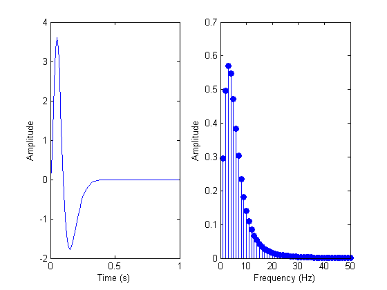
As you can see in the plot of fourier spectrum, this filter has a maximum sesnsitivity to frequencies around 3 Hz. You can also see this from the shape of the impulse response. It wiggles up and down one cycle in about 1/3 of a second, which is 3Hz. A convolution with a 3Hz sinusoid will produce the largest response.

An example: the hemodynamic response function

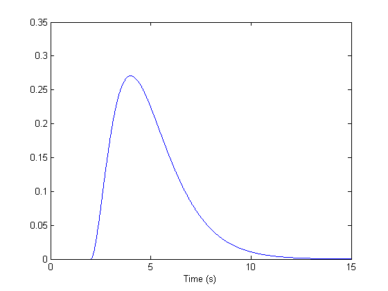
Functional MRI (fMRI) measures changes in blood flow and oxygenation associated with the underlying neuronal response. The most common method for analyizing fMRI data uses the 'general linear model' that assumes that the 'hemodynamic coupling' process acts as a linear shift-invariant filter. Back in 1996 we tested this idea and found that the impulse response function acts like a cascade of leaky integrators with these typical parameters:

k = 1; %seconds
nCascades = 3;
delay = 2; %seconds

Which looks like this:

dt = .01;  %step size (seconds)
maxt = 15;  %ending time (seconds)
t = 0:dt:(maxt-dt);

hdr = gamma(nCascades,k,t-2);

clf
plot(t,hdr);
xlabel('Time (s)');

One kind of fMRI experimental design is a 'blocked design' where two conditions alternate back and forth. A Typical period for a blocked design is something like 25 seconds. If we assume that the neuronal response is following the stimulus closely in time (compared to the hemodyanmic response), the neuronal response might look something like this:

dt = .01;  %step size (seconds)
maxt = 120;  %ending time (seconds)
t = 0:dt:(maxt-dt);
period = 25; %seconds
s = sign(sin(2*pi*t/period));

y = conv(s,hdr)*dt;
y = y(1:length(t));

plotResp(t,s,y);

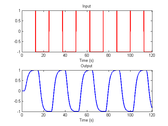
The output is the expected shape of the fMRI response. Many software packages will use a convolution with the stimulus design to produce an expected response like this as a template to compare to the actual fMRI data. This template is correlated with each voxel's time-series to produce a number between zero and 1, where 1 is a perfect fit. This produces a 'parameter map' that can tell us which brain areas are responding as expected to the experimental paradigm.

Published with MATLAB® 7.6