Lesson

Lesson 13: Event-Related fMRI and 'Deconvolution'
Deconvolution
Efficiency of a stimulus sequence
m-sequences
Multiple event types
Other regressors:
Exercises

Lesson 13: Event-Related fMRI and 'Deconvolution'

Since the expected fMRI response is the convolution of the impulse response with the neuronal response, it's possible work backwards and estimate the hemodynamic response that best predicts a measured fMRI signal. This is essentially undoing the convolution process, or 'deconvolution'.

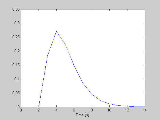
Let 'h' be be the vector representing the hemodynamic response function, and 's' be the vector of zeros and ones containing the time-points when 'events' occured. A linear system predicts that the fMRI response, y, is the convolution of the h and s. Here's an example:

dt = 1;  %step size (seconds)
maxt = 15;  %ending time (seconds)
th = 0:dt:(maxt-dt);
n = length(th);  %n is the length of the hdr.

k = 1; %seconds
nCascades = 3;
delay = 2; %seconds
h = gamma(nCascades,k,th-delay)';  %make it a column vector

figure(1)
clf
plot(th,h);
xlabel('Time (s)');

% Here's the event sequence:
maxt = 255;  %ending time (seconds)
t = 0:dt:(maxt-dt);
m = length(t);  %m is the length of the event sequence

prob = .5;  %probability of an event for each time point.
s = floor(rand(1,m)+prob)';
y = conv(s,h)*dt;
y = y(1:m);

Deconvolution

Suppose, now, that we only know the response, y, and our event sequence, s. How can we reconstruct the hemodynamic response? Specifically, if the hdr has, say, 15 time points, then we need to find the best 15 numbers that will predict our fMRI response. A brute-force method would be to use a search algorithm to find the best 15 numbers that minimizes the error between the predicted and the measured fMRI response. Fortunately, there's an easier and more efficent way using linear algebra.

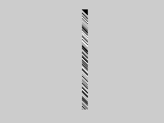
The trick is to think of this is a giant linear algebra problem with 15 unknowns and n knowns, where n is the length of the fMRI response. We can see that this is a linear algebra problem by noting that convolution can be conducted through matrix multiplication (indeed, this is how matlab does it). This is done by transforming our stimulus sequence, s, into a 'design matrix' X that, when multipied by the hdr, performs the convolution.

Remember that convolution is the process of multiplying shifted copies of the hdr with the input and adding. Equivalently (since convolution is commutative) this can be done with shifted copies of the input instead.

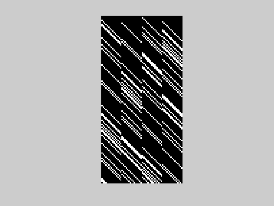
The columns of the design matrix, X, aregenerated by successive shifts of the stimulus, like this:

X = zeros(m,n);
temp = s;
for i=1:n
    X(:,i) = temp;
    temp = [0;temp(1:end-1)];
end

figure(1)
clf
imagesc(X)
axis equal
axis off
colormap(gray)

convolution of s and h is done by multiplying the design matrix X and h (as a column vector):

r = X*h;

% we can compare this to matlab's convolution by taking the norm of the
% difference between the two vectors.  A small number means they're the
% same (the norm of a vector is the square root of the sum of squares).

rconv = conv(s,h); rconv = rconv(1:m);
norm(r-rconv)

ans =

  1.4327e-015

Here's where the linear algebra comes in. if r = X*h, then if this were normal algebra we could solve for h by dividing r by X (h = r/X). When r and h are vectors and X is a matrix, this 'division' is done by finding the least-squared solution with the 'psueudo-inverse'. How this works is beyond our scope (but elegant). Details can be found in most engineering and linear algebra textbooks.

PX = inv(X'*X)*X';

% Matlab has its own function that does this called 'pinv'

PX = pinv(X);

hest = PX*r;

We'll use 'norm' again to compare hest to h:

norm(hest-h)

ans =

  4.1852e-016

What did we just do? To recap, we made up a hemodynamic response function, h, convolved it with a random stimulus sequence, s, to get an fMRI response, r. We then did the whole thing in reverse and reconstructed h from r and s by deconvolving via the pseudo-inverse.

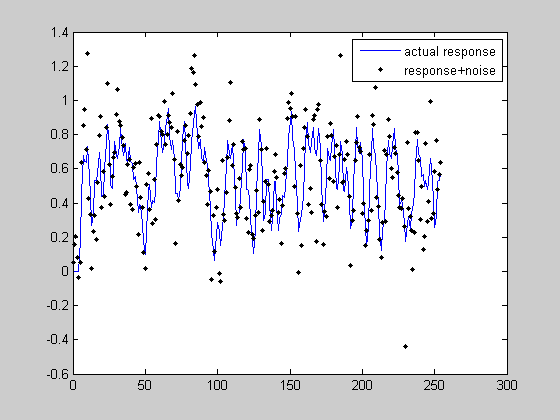
Real fMRI data is noisy. Let's add independently and identically distributed ('iid') noise to the response and see how it affects our ability to reconstruct the hemodynamic response

noiseSD = .2;
rnoise = r+noiseSD*randn(m,1);

figure(1)
clf

plot(t,r,'b-');
hold on
plot(t,rnoise,'k.');
legend({'actual response','response+noise'});

hest = PX*rnoise;

figure(2)
clf
plot(th,h,'b-');
hold on
plot(th,hest,'k.','MarkerFaceColor','k')
xlabel('Time');
legend({'actual hdr','reconstructed hdr'});

norm(hest-h)

ans =

    0.1067

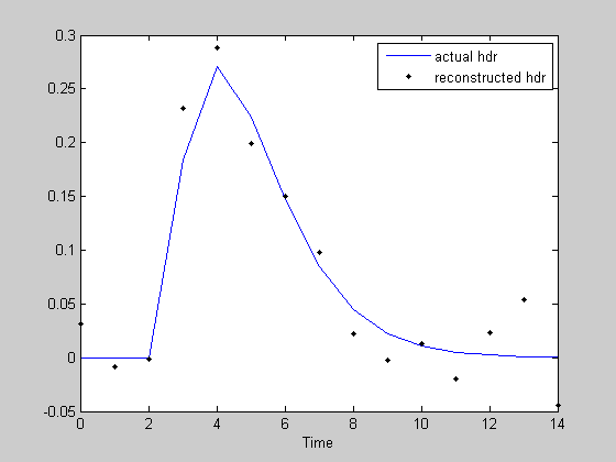
You might be surprised how robust our estimate of the hdr is considering how much noise we added to the response. This is because we have so many knowns to help constrain the number of unknowns. As you can guess, the longer the event sequence, the better we will be at estimating the true hdr.

Go ahead and play with the magnitude of the noise (noiseSD) and see how it affects the estimate of the hdr.

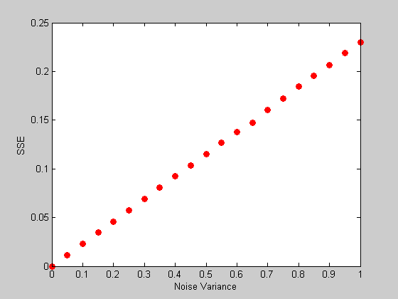
It turns out that the average value of norm(h-hest) grows in proportion to the standard deviation of the added noise (or equivalently the sums of squared error grows in proportion to the variance of the noise) We can demonstrate this with a simulation:

noiseVar = linspace(0,1,21);  %list of noise variances
nReps = 5000;  %number of repetitions per noise variance level

err=  zeros(nReps,length(noiseVar));
for i=1:length(noiseVar)
    for j=1:nReps
        rnoise = r+sqrt(noiseVar(i))*randn(m,1);
        hest = PX*rnoise;
        err(j,i) = norm(hest-h)^2;
    end
end

meanErr=  mean(err);

figure(1)
clf
plot(noiseVar,meanErr,'ro','MarkerFaceColor','r');
xlabel('Noise Variance');
ylabel('SSE');

Efficiency of a stimulus sequence

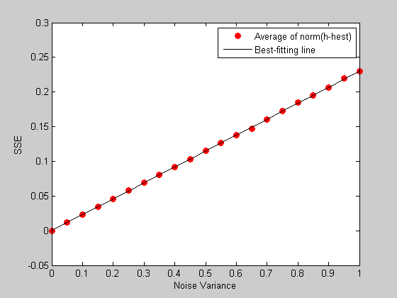
The slope of this line tells us something about the way the ability to reconstruct the hdr falls apart with increasing noise. A lower slope is better. Different event sequences will have different slopes. Try it out yourself by running the program with a different kind of sequence.

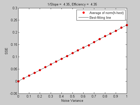
Since low slopes are good, the inverse of the slope has a special meaning, called the 'efficiency' of the event sequence. Let's calculate this number from our simulated data:

%Fit a line to the data
p = polyfit(noiseVar,meanErr,1);
bestLine = polyval(p,noiseVar);
hold on
plot(noiseVar,bestLine,'k-');
legend({'Average of norm(h-hest)','Best-fitting line'});

It also turns out that there's a simple way of calculating the efficiency without a simulation. Here's how:

E = 1/trace(inv(X'*X));

The trace of a matrix is the sum of its diagonals. The derivation of this equation is, once again, beyond the scope of this lesson (and beyond the scope of my full understanding). But let's just assume it's true. This number should be close to the inverse of the slope from the simulation:

title(sprintf('1/Slope = %5.3g, Efficiency = %5.3g',1/p(1),E));

So we now have an easy way to assess how well a given event sequence will be able to reconstruct the hemodynamic response (assuming that the 'hemodynamic coupling' process is linear, and that noise is additive, which can't be completely right).

Here's something interesting: the calculation of efficiency doesn't depend on the shape of the hdr. It's kind of an amazing fact if you think about it. We could have chosen any crazy shape for the hdr and the ability to reconstruct it from noise data will be exactly the same. This is a very convenient fact, too, since we don't know the actual shape of the hdr (it's what we're trying to find out).

m-sequences

There is one kind of sequence that has the greatest efficiency - the m-sequence. M-sequences (or maximum-length shift register sequences) were originally developed about 50 years ago and have been used in encryption, error-correcting codes - any time you want to generate a signal that is minimally corruptible by noise. Generation of m-sequences is not intuitive - it involves prime numbers and modulo arithmetic. But the result is a sequence that has a zero autocorrelation function. I've provided a function 'mseq' that generates these sequences for you. 'mseq' takes in a minimum of two parameters. The first is the number of event types (here we've only talked about zeros and ones, so the number is 2, since blank trials count as an event type). The second is a 'power value' that determines the length of the sequence, which will be nTypes^(powerVal-1).

A more thorough discussion of m-sequences applied to event-related fMRI can be found here:

G.T. Buracas and G.,M. Boynton (2002), "Efficient Design of Event-Related fMRI Experiments Using M-Sequences" , NeuroImage 16, 801-813

powerVal = 8;
ms = mseq(2,powerVal);

X = zeros(m,n);
temp = ms;

%Calculate the efficiency:
for i=1:n
    X(:,i) = temp;
    temp = [0;temp(1:end-1)];
end
Emseq = 1/trace(inv(X'*X));

disp(sprintf('Efficiency of m-sequence: %5.3g',Emseq));

%This number should be greater than our example random sequence (it had
%better be anyway).

Efficiency of m-sequence:  4.54

Multiple event types

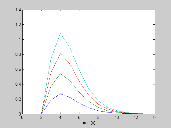
Event-related fMRI often involves more than one type of stimulus in a given scan. Stimuli may include, for example, a parametric range of stimulus values, like contrast. Or they may be different cognitive or attentive tasks. There's an easy way to incorporate multiple event types into your design and analysis. The trick is to simply concatenate the separate design matrices horizontally (with zeros and ones in each matrix). The resulting estimate of the hemodynamic response will be a single vector with the estimate of the response to each condition in succession. We'll demonstrate this by creating four 'fake' hdrs, generating a response with convolution, adding noise, and reconstructing the hdrs.

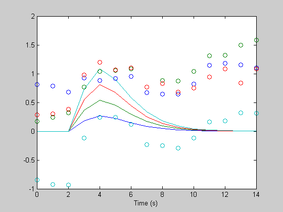
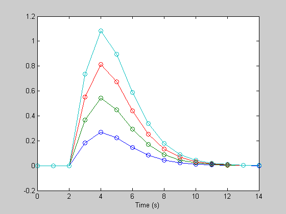
amps = [1,2,3,4];  %amplitudes of the hdr for the four event types (e.g. for increasing stimulus contrast).

h = zeros(n,4);
for i=1:4
    delay = 2; %seconds
    h(:,i) = amps(i)*gamma(nCascades,k,th-delay)';  %make it a column vector
end

figure(1)
clf
plot(th,h);
xlabel('Time (s)');

%get an m-sequence with four event types - plus null events.  This vector
%will have values from 0 to 4 corresponding to what happens on each time
%step.

s = mseq(5,3);
m = length(s);
t = 0:dt:(m-1);

%Generate a concatenated design matrix
X = [];
for j=1:4
    Xj = zeros(m,n);
    temp = s==j;

    for i=1:n
        Xj(:,i) = temp;
        temp = [0;temp(1:end-1)];
    end
    X = [X,Xj];
end

figure(1)
clf
imagesc(X)
axis equal
axis off
colormap(gray)

r = X*h(:);

%add noise
noiseSD = .25;
rNoise = r+noiseSD*randn(size(r));

hest = pinv(X)*rNoise;

The resulting hdr estimates are all in one long vector. To show them in the form of the original hdr we can reshape this vector back into an nx4 matrix:

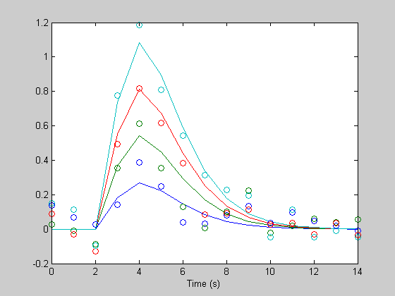
hest = reshape(hest,n,4);

figure(1)
clf
plot(th,h);
hold on
plot(th,hest,'o');
xlabel('Time (s)');

Other regressors:

In addition to the additive-type noise, fMRI signals are contaminated with low-frequency noise, often characterized as linear trend either up or down, along with a large y-intercept. The y-intercept is just the mean of the image which doesn't carry any functional information (the mean is a T2-weighted image that contains structural information, however). The linear trend is more troublesome - it can dominate the time-course of a voxel when viewed by eye, yet its causes aren't well understood. So we just subtract it out. Scary? Yes.

It's easy to remove these trends in the same step as the deconvolution process. This is because each column in the design matrix 'X' represents the time-course to be explained by each free parameter. The first column is for the first time-point in the hdr, for example. To regress out a DC, then, we simply add a column of 1's to the end of the design matrix. The resulting last parameter will be the best-fitting parameter for the DC (which will be the mean). Similarly, if we add a ramp to X, the regressor will be the best fitting scale factor that makes that ramp fit the data. We don't use these parameters, instead by adding them to the matrix their influences get factored, or regressed out.

First, let's see how a DC and trend screws up our estimation of the hdr before regressing them out:

rtrend = r+100 + linspace(0,10,m)';

figure(1)
clf
plot(t,rtrend);
xlabel('Time (s)');

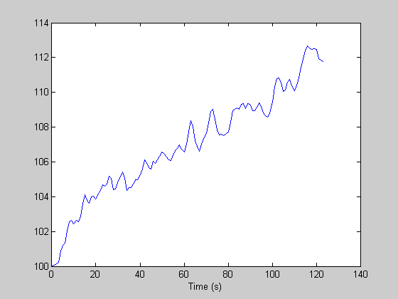
Now THAT looks more like fMRI data. Here's the estimated hdr:

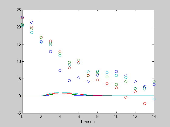
hest = pinv(X)*rtrend;
hest = reshape(hest,n,4);

figure(1)
clf
plot(th,h);
hold on
plot(th,hest,'o');
xlabel('Time (s)');

What a mess. Let's add a column of ones to X to deal with the DC:

X(:,n*4+1) = ones(m,1);
hest = pinv(X)*rtrend;

The DC regressor is the last element in hest. It should be about 100

dc = hest(end)

hest = reshape(hest(1:n*4),n,4);

figure(1)
clf
plot(th,h);
hold on
plot(th,hest,'o');
xlabel('Time (s)');

dc =

  100.0460

Better, but we have to get rid of the linear trend, too

X(:,n*4+2) = linspace(0,1,m)';

hest = pinv(X)*rtrend;
lowFac = hest(end-1:end);
hest = reshape(hest(1:end-2),n,4);

figure(1)
clf
h1=  plot(th,h);
hold on
h2= plot(th,hest,'o');
xlabel('Time (s)');

It's back. You can see how important it is to get rid of these factors - the DC is essential because the deconvolution process only works if you either remove the DC via regression, or if you remove it ahead of time by subtracting out the mean.

In this discussion of deconvolution, we assumed that the fMRI response is a linear transformation of the neuronal response with iid noise. It's known that the noise in the signal has temporal correlations in it. For a discussion on how to deal with that via deconvolution, see an excellent paper by Anders Dale:

Dale, A. (1999) "Optimal Experimental Design for Event-Related fMRI", Human Brain Mapping 8:109–114

Exercises

1) The efficiency of a random sequence depends on the probability of an event occuring on a given trial (the variable 'prob' above). Plot a graph of efficiency as a function of prob (between 0 and 1) to see what probability yields the most efficient sequence.

2) Generate a bunch of random 50% probability event sequences to see if you get anything close to the efficiency of an m-sequence. Do you think this random procedure is worthwhile? What are its advantages?

3) Removing the DC and linear trend is one way of removing 'low-frequency' factors in the fMRI signal. Using what we learned from Lesson 12, how would you remove low-frequency stuff using the frequency domain? Many fMRI software packages do this sort of thing.

Contents