Lesson

Lesson 14: The 2-D FFT
Creating images using x and y 'meshgrid' matrices
The 2-D FFT
fftshift
zero-padding
plotFFT2
Low-Pass filtering
Band-pass filtering of an impulse
Statistics of natural images
Spatial Frequencies of Natural Images
Orientations in Natural Images
Exercises

Lesson 14: The 2-D FFT

This lesson will cover how to use matlab's 'fft2' function to look at the representation of 2-D images in the frequency domain.

clear all

Creating images using x and y 'meshgrid' matrices

This was covered in the 'intro' version of this course, but we'll review it here. First we'll define some variables that will determine the parameters for our images. 'wDeg' will be the width and height of the image in degrees of visual angle, and 'nPix' will be the number of pixels in a row or column. To keep things simple, all images will be square nPix by nPix matrices.

wDeg = 1;  %size of image (in degrees)
nPix = 200;  %resolution of image (pixels);

[x,y] = meshgrid(linspace(-wDeg/2,wDeg/2,nPix+1));
x = x(1:end-1,1:end-1);
y = y(1:end-1,1:end-1);

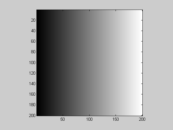
We can view the 'x' matrix as an image with matlab's imagesc function:

figure(1)
clf
imagesc(x);
axis equal
axis off
colormap(gray);

I've provided a simple function 'showImage' that runs the lines above, since we'll be doing this a lot in this lesson:

showImage(x);

showImage takes in optional 'x' and 'y' matrices to use for the axes:

showImage(x,x,y);

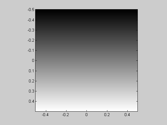
You can guess what the 'y' matrix looks like:

showImage(y,x,y);

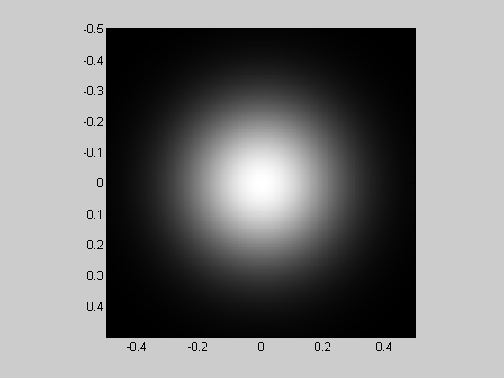
These 'x' and 'y' matrices can be used to generate a wide range of images without any for-loops. For example, here's a Gaussian.

sigma = .25;  %width of Gaussian (1/e half-width)
Gaussian = exp(-(x.^2+y.^2)/sigma^2);
showImage(Gaussian,x,y);

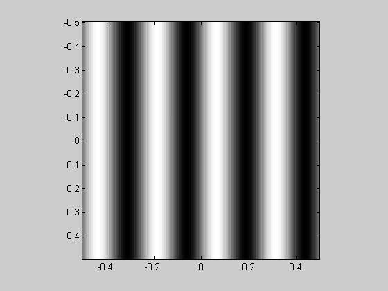
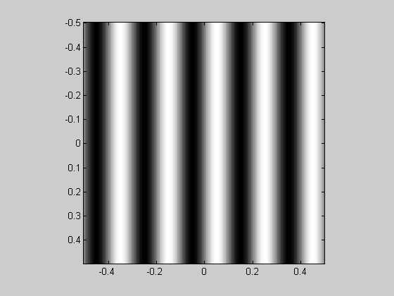
A 'grating' can be generated easily too. The orientation of the grating is incorporated by combining the 'x' and 'y' matrices to make a ramp that increases in the desired direction:

orientation = 90;  %deg (counter-clockwise from horizontal)
sf = 4; %spatial frequency (cycles/deg)

ramp = sin(orientation*pi/180)*x-cos(orientation*pi/180)*y;

grating = sin(2*pi*sf*ramp);
showImage(grating,x,y);

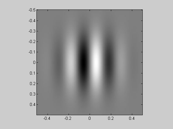
You've probably guessed what's next. A Gabor is the product of a Gaussian and a grating.

Gabor = grating.*Gaussian;
showImage(Gabor,x,y);

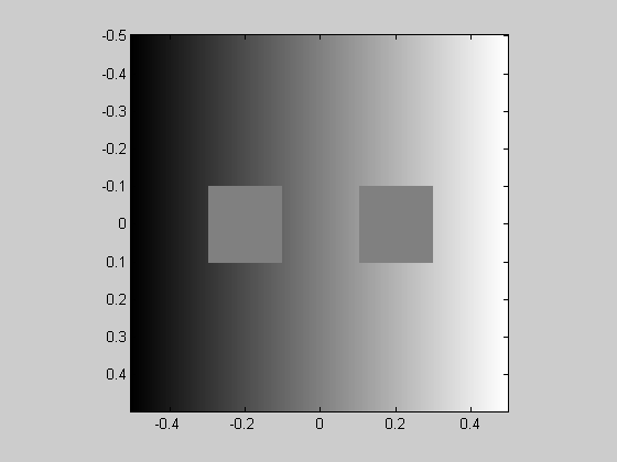
As a short detour, it's easy to generate all sorts of fun images with the 'x' and 'y' matrices. Here's the classic simultaneous contrast illusion made by placing two gray boxes on the 'x' matrix.

img = x;
img(x<-.1 & x>-.3 & abs(y)<.1) = 0;  %left box
img(x> .1 & x< .3 & abs(y)<.1) = 0;  %right box
showImage(img,x,y);

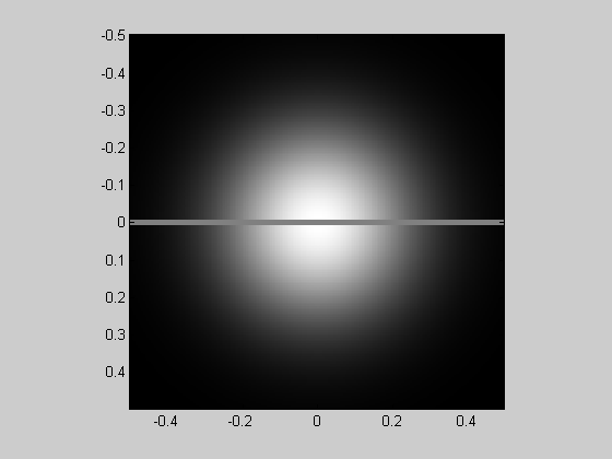
Here's another version of the simultaneous contrast illusion by putting a gray strip through the 'Gaussian' image.

img = Gaussian;
img(abs(y)<.01) = .5;
showImage(img,x,y);

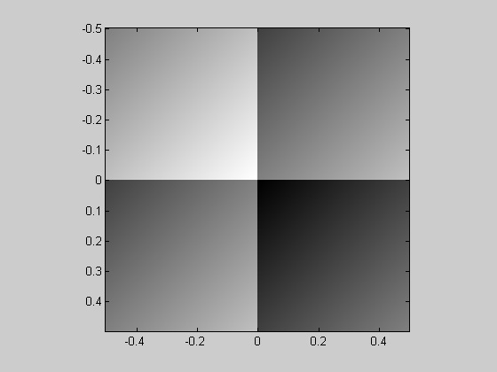
I like this simple one that I made up. It's a 4x4 array of grayscale ramps, but it looks like four uniform patches:

img = mod(x,1)+ mod(y,1);
showImage(img,x,y)

And so on.

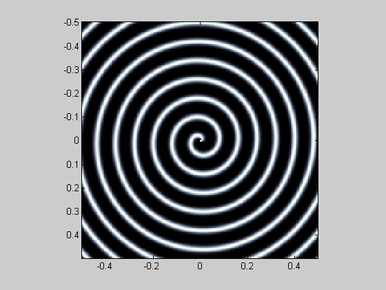
img  = cos(atan2(y,x)+ 25*pi*sqrt(x.^2+y.^2));
img = ((img+1)/2).^4;

showImage(img,x,y);
colormap(bone)

The 2-D FFT

But we digress... back to filtering and FFTs. Remember that any 1-D time-series can be represented as a sum of sinusoids. This fact generalizes to 2-D matrices where any image can be represented as a sum of gratings. These gratings will vary in spatial frequency (cycles/image), amplitude phase, and orientation. Remember that a n-element vector can be represented by n/2 sinusoids. Interestingly, an nxn pixel image (n^2 pixels) can be faithfully represented by n^2/4 gratings. This is because each grating can be described with four parameters (amplitude and phase in each of the x and y dimensions).

There is a fast Fourier transform for two dimensions that is implemented with Matlab's 'fft2' function. To interpret the output, we'll start with the fft2 run on our grating stimulus, which should produce a 'spike' in the frequency domain:

F = fft2(grating);

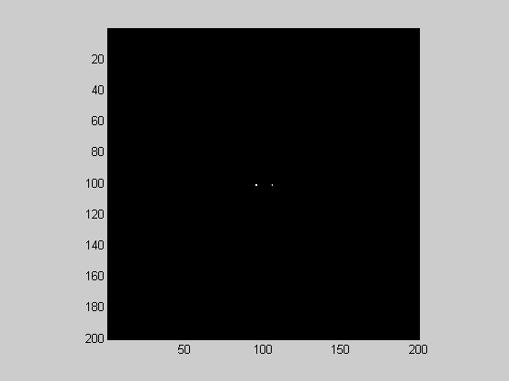
Once again it's full of complex numbers. Each one represents the amplitude and phase of a grating. We can view the amplitudes as an image:

showImage(abs(F));

Where's the 'spike'? It's up in the top row. By default the gratings represented in the fft2 increase in spatial frequency along the x-dimension and y-dimension, starting in the upper-left corner. In fact, since this grating only varies in the x-dimension, the first row of F should look like the fft:

figure(2)
clf
stem(0:9,abs(F(1,1:10)));
xlabel('Cycles/image');

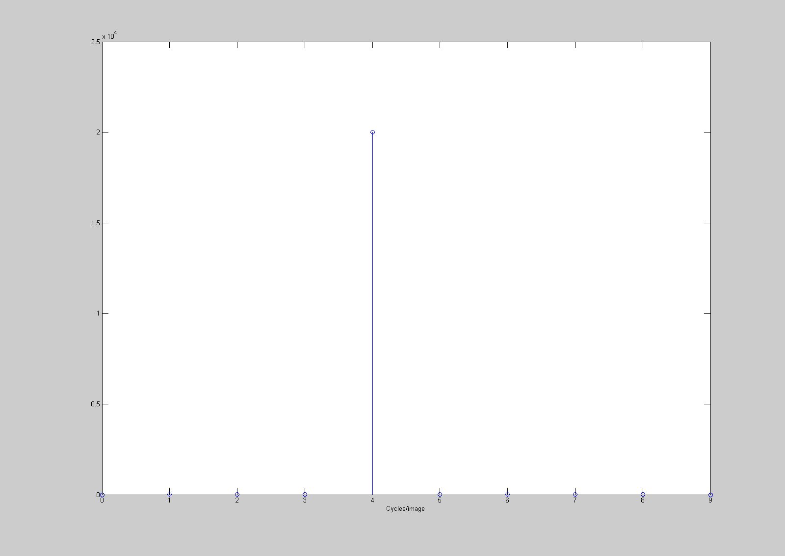
Since the spatial frequency was 4 cycles/deg and the image spanned 1 deg, the spike is in the fifth entry, corresponding to 4 cycles/image. You can now easily predict what the fft2 of a horizontal grating will be for any frequency. Try it out for yourself.

fftshift

Since the low spatial frequencies end up in the corners from fft2, a common representation is to rearrange the quadrants so that the corners meet up in the center of the image. This way the center of the image represents the lowest frequencies. This is done with Matlab's 'fftshift':

figure(1)
F = fftshift(F);
showImage(abs(F));

With the 1-D fft we ignored the 'negative' frequencies. However, with the 2-D fft, it's customary to show both the positive and negative frequencies. Hence the two 'spikes' in the fft2 of the grating stimulus - one at 4 c/deg and one at '-4' c/deg.

We generated an oriented grating by taking the sine of an oriented ramp. The ramp was generated as a linear combination of the 'x' and 'y' matrices, which shows us that the cross sections of an orientated grating along the x or y dimensions are sinusoids modulating at frequencies based on this linear combination. For example, if the orientation is 30 degrees, the grating is made like this:

orientation = -45;  %deg (counter-clockwise from vertical)
sf = 5; %spatial frequency (cycles/deg)

ramp = cos(orientation*pi/180)*x - sin(orientation*pi/180)*y;

grating = sin(2*pi*sf*ramp);
figure(1)
showImage(grating,x,y);

The spatial frequency along the x and y-dimensions are:

sfx = sf*cos(orientation*pi/180)
sfy = sf*sin(orientation*pi/180)

sfx =

    3.5355


sfy =

   -3.5355

This means that the 'spike' in the fft2 of an oriented grating will be found at (sfx, sfy):

F = fftshift(fft2(grating));
showImage(abs(F));

Let's zoom in on the center:

figure(1)
showImage(abs(F(nPix/2-10:nPix/2+10,nPix/2-10:nPix/2+10)));

You'll see that there are two spikes, just like for the 1-D fft. For the 2-D fft, the spikes will always be found at mirror image locations reflected across the origin. In this example we have a spike at about (2.8, -2.8) cycles/image and it's mirror at (-2.8,2.8) cycles/image. The reason why the spikes are spread out is because 2.8 isn't an integer number.

zero-padding

Often the most interesting part of the frequency spectrum in an image is near the low frequencies, as in the example above. A nice way to view the spectrum at these low frequencies is to increase the size of the image before the fft by placing it in the middle of a bigger zeroed out matrix:

padFac = 5;
F =fftshift(fft2(grating,nPix*padFac,nPix*padFac));
center = round( nPix*padFac/2-nPix/2):round( nPix*padFac/2+nPix/2);

F = F(center,center);
showImage(abs(F));

%Why does this work?  If we, say, double the size of the image, then the
%resulting frequencies in the fft are going to be 1,2,3... cycles per
%image, which corresponds to frequencies of 0.5,1,1.5,... cycles per image
%for the original image.  Thus, the resolution of our frequency spectrum
%has been effectively increased by zero-padding.

plotFFT2

I've provided a function 'plotFFT2' that is like 'plotFFT' but for images. It takes in as arguments the image, x and y matrices (for labeling the axes), a factor for zero-padding, and the maximum spatial frequency for cropping the image. Here's an example

figure(1)
clf
plotFFT2(grating,x,y,4,10);

In this example, the 200x200 image 'grating' was padded by a factor of four to make it a 800x800 image. The axes are set to cut off at +/- 10 c/deg.

We're now ready to look at the fft2 of more interesting images.

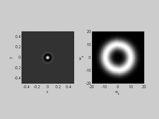
The fft2 of a Gaussian is a Gaussian:

sigma = .05;  %width of Gaussian (1/e half-width)
Gaussian = exp(-(x.^2+y.^2)/sigma^2);

plotFFT2(Gaussian,x,y,5,25);

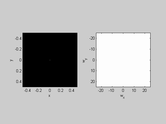
Play with the width of the Gaussian by changing 'sigma' and see if you get what you'd expect from what we learned from the 1-D fft.

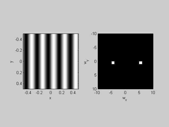
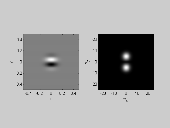
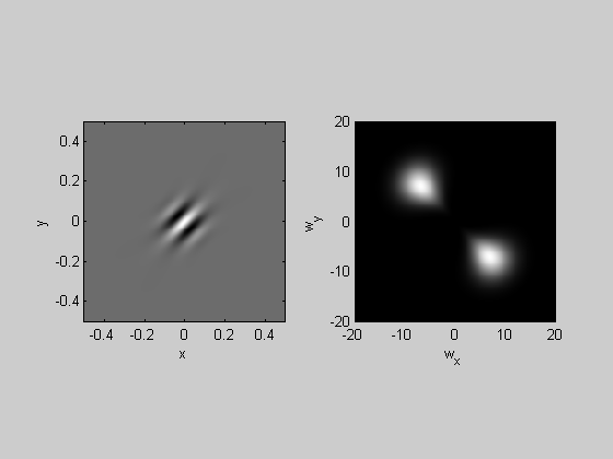
A Gabor is a grating multiplied by a Gaussian. The fft will be two Gaussians, centered at the frequency of the grating.

sigma = .1;  %width of Gaussian (1/e half-width)
orientation = 0;  %deg (counter-clockwise from vertical)
sf = 5; %spatial frequency (cycles/deg)

Gaussian = exp(-(x.^2+y.^2)/sigma^2);
ramp = sin(orientation*pi/180)*x-cos(orientation*pi/180)*y;
grating = sin(2*pi*sf*ramp);
Gabor = Gaussian.*grating;

plotFFT2(Gabor,x,y,5,25);

A Plaid is the sum of two gratings. Since the fft is linear, the fft will show 'spikes' for each of the grating components.

sigma = .1;  %width of Gaussian (1/e half-width)
orientation = -45;  %deg (counter-clockwise from vertical)
sf = 10; %spatial frequency (cycles/deg)

Gaussian = exp(-(x.^2+y.^2)/sigma^2);
ramp = sin(orientation*pi/180)*x-cos(orientation*pi/180)*y;
grating = sin(2*pi*sf*ramp);
plaid = (grating+flipud(grating))/2;

plotFFT2(plaid,x,y,5,20);

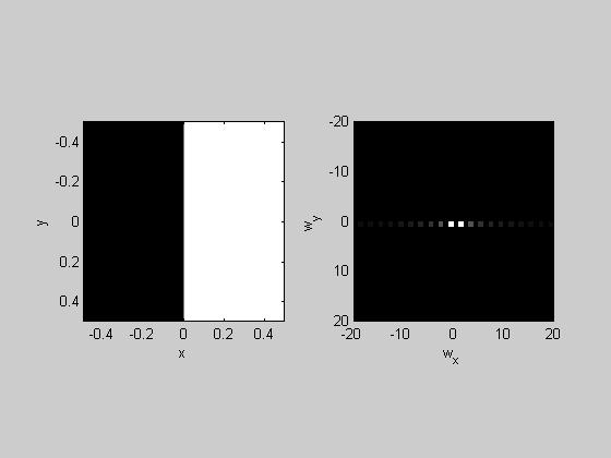
Edge:

img = sign(x);
plotFFT2(img,x,y,1,20);

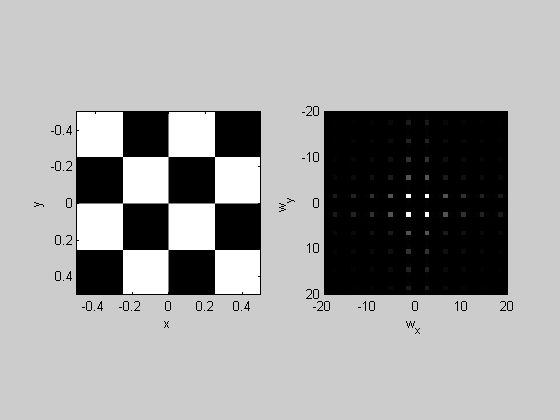
%Checkerboard:

img = sign(sin(4*pi*x).*sin(4*pi*y));
plotFFT2(img,x,y,1,20);

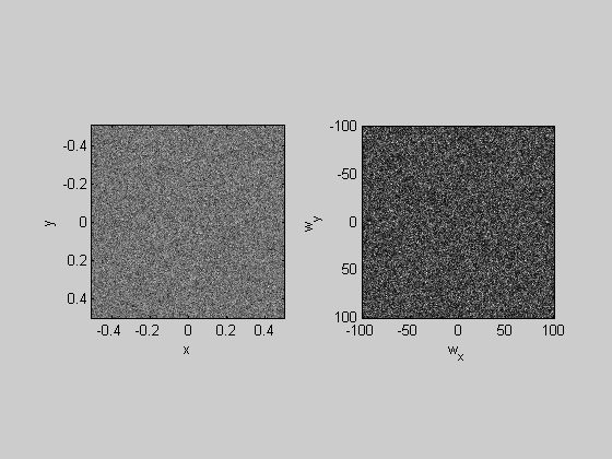
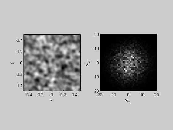
%Noise

noise = randn(nPix);
plotFFT2(noise,x,y);

Low-Pass filtering

We can low-pass an image by multiplying the amplitudes in the frequency domain by a Gaussian centered at zero frequency. Just like for the fft, the output of fft2 has complex numbers that are scaled in a funny way. I've provided a function 'myfft2' that returns a structure containing the amplitudes and phases for each frequency in the image. 'myifft2' takes the inverse fft (using matlab's 'ifft2') to get the filtered image back.

k=1;
F = myfft2(noise,x,y,k);

% multiply the amplitudes by a Gaussian:
sigma = 10;  %c/deg
Gaussian = exp(-F.sf.^2/sigma^2);
F.amp = F.amp.*Gaussian;

lowPassImg = myifft2(F);

plotFFT2(lowPassImg,x,y,k,20);

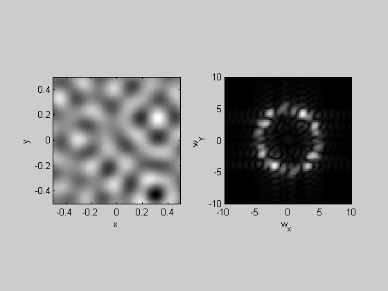
Band-Pass filtering is similar, but using a Gaussian 'envelope' that is centered at some nonzero spatial frequency:

k=4;
F = myfft2(noise,x,y,k);
sigma = .5;  %c/deg
centerFreq = 5; %c/deg
Gaussian = exp(-(F.sf-centerFreq).^2/sigma^2);
F.amp = F.amp.*Gaussian;

lowPassImg = myifft2(F);

plotFFT2(lowPassImg,x,y,k,10);

Orientation filtering can be done by multiplying the amplitudes by a window in the angle dimension. A good way to do this is with the 'Von Mises' function that deals with the circularity of the angle dimension:

k=4;
F = myfft2(noise,x,y,k);
sigmaAng = 10;  %deg
centerAng = 0; %c/deg

%vonMises function
VonMises = exp(-sigmaAng*cos(pi*(2*(F.angle-centerAng))/180));
F.amp = F.amp.*VonMises;

angleImg = myifft2(F);

plotFFT2(angleImg,x,y,k);

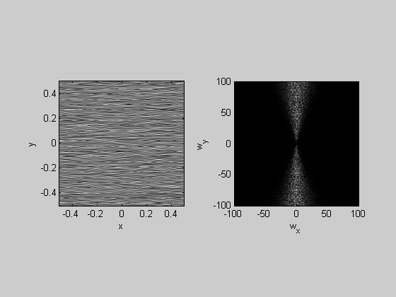
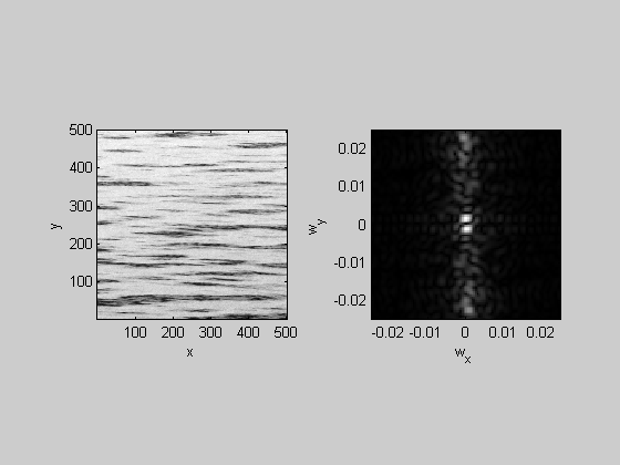
%Looks like water.  I just took a picture of some water for comparison:

img = imread('water.JPG');
figure(2)
clf
image(img);
axis equal
axis tight

l = 1000;
t = 1000;
nPix = 500;

hold on
plot([l,l+nPix-1,l+nPix-1,l,l],[t,t,t+nPix-1,t+nPix-1,t],'r-','LineWidth',2);

img = mean(img,3);

%crop
img = img(t:t+nPix-1,l:l+nPix-1);
img = flipud(img);

img= img-mean(img(:));

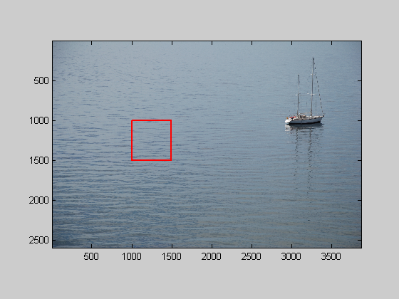
Show the cropped image and it's fft in figure 1

figure(1)
plotFFT2(img,[],[],4,.025);

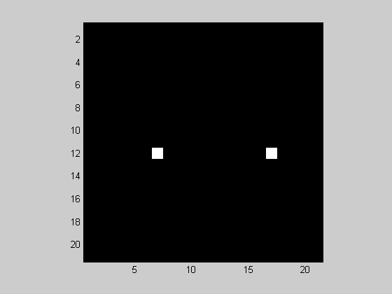
Band-pass filtering of an impulse

Back in lession 11, when we were working with the 1-D fft, we created our first 'filter' by band-passing the fft of an impulse and sending the result back into the time-domain. We'll do this again but in 2-D to create a band-pass filter for images.

nPix = 200;
k=4;

Take the Fourier transform of the impulse:

img= zeros(nPix);
img(nPix/2,nPix/2) = 1;
F = myfft2(img,x,y,k);

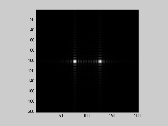
Attenuate the amplitudes by a Gaussian

sigma = 4;  %c/deg
centerFreq = 10; %c/deg
Gaussian = exp(-(F.sf-centerFreq).^2/sigma^2);
F.amp = F.amp.*Gaussian;

Take the inverse fft to see the result in the space-domain:

filt = myifft2(F);
plotFFT2(filt,x,y,k,20);

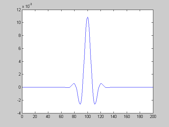
Here's a cross-section of the middle of the matrix 'filt'. You'll see that it has the classic shape of a 'center/surround' filter. This like an LGN receptive field which can be thought of as a band-pass filter.

figure(2)
clf
plot(filt(end/2,:));

Next we'll both band-pass an impulse and restrict it's range of orientations:

k=5;
img= zeros(nPix);
img(nPix/2,nPix/2) = 1;

F = myfft2(img,x,y,k);
sigma = 4;  %c/deg
centerFreq = 10; %c/deg
sigmaAng = 2.5;  %deg
centerAng = 45; %deg

%vonMises function
VonMises = exp(-sigmaAng*cos(pi*(2*(F.angle-centerAng))/180));
F.amp = F.amp.*VonMises;

Gaussian = exp(-(F.sf-centerFreq).^2/sigma^2);
F.amp = F.amp.*Gaussian.*VonMises;
filt = myifft2(F);
plotFFT2(filt,x,y,k,20);

Statistics of natural images

There is a lot of research on the properties of natural images, and much of this is done through analysis in the frequency domain. Here we'll investigate the distribution of amplitudes with respect to spatial frequency and orientation.

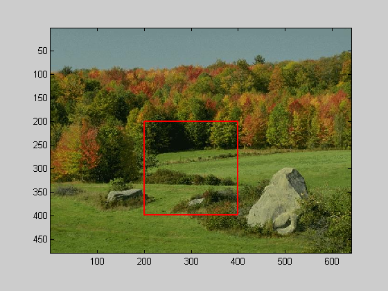
First we'll load in a 'natural' image:

k=5;
img = imread('forest.JPG');
%img = imrotate(img,-45,'crop');

%show the image in figure 2
figure(2)
clf
image(img);
axis equal
axis tight

%crop the image to 200x200 pixels
l = 200;
t = 200;
nPix = 200;

%draw the crop as a red square in figure 1
hold on
plot([l,l+nPix-1,l+nPix-1,l,l],[t,t,t+nPix-1,t+nPix-1,t],'r-','LineWidth',2);

%collapse across the r,g,b dimensions
img = mean(img,3);

%crop the image
img = img(t:t+nPix-1,l:l+nPix-1);
img = flipud(img);

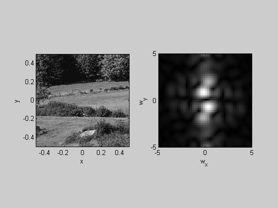
Show the cropped image and it's 2-D fft:

figure(1)
plotFFT2(img-mean(img(:)),x,y,k,5);

Spatial Frequencies of Natural Images

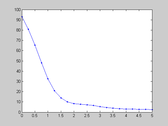
An interesting property of natural images is that they have a frequency spectrum that falls off roughly as the inverse of the spatial frequency (1/f). We can see this by summing up the amplitudes within a sliding Gaussian window across frequencies:

centerList = linspace(0,5,21);
sigma = .5;

F = myfft2(img,x,y,4);

amp = zeros(size(centerList));
for i=1:length(centerList)
    Gaussian = exp(-(F.sf-centerList(i)).^2/sigma^2);
    amp(i) = sum(F.amp(:).*Gaussian(:))/sum(Gaussian(:));
end

figure(3)
clf
plot(centerList,amp,'b.-');

Orientations in Natural Images

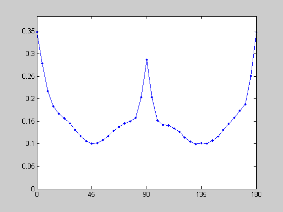
Natural and man-made scenes tend to have more vertical and horizontal 'stuff' in them. This fact has been used as an argument for why the visual system shows an 'oblique effect' - greater sensitivity to the cardinal orientations, and a greater number of neurons tuned to these orientations. Let's look at this in our natural image using a sliding Von Mises function to count up the amount of oriented amplitude within a given window:

centerList = linspace(0,180,41);
sigmaAng = 90;

F = myfft2(img,x,y,4);

amp = zeros(size(centerList));
for i=1:length(centerList)

    VonMises = exp(-sigmaAng*cos(pi*(2*(F.angle-centerList(i)))/180));
    amp(i) = sum(F.amp(:).*VonMises(:))/sum(VonMises(:));
end

figure(3)
clf
plot(centerList,amp,'b.-');
set(gca,'YLim',[0,max(amp)*1.1]);
set(gca,'XTick',[0:45:180]);

Exercises

1) Find some images on the web and check to see if their spatial frequency profile falls of as the inverse of frequency.

2) See if you can find any natural images on the web that don't have the 'oblique effect'.

3) The digitization process used by digital cameras can add artifacts to images, including vertical and horizontal components in frequency space. If you have a camera, you can test for this by taking images of the same scene and rotating the camera by a different angle each time. The pattern of orientations in the image should shift accordingly, and there should be no consistent 'spike' at 0 or 90 degrees.

Contents