Lesson 15: Filtering 2-D images

This lesson is all about how convolving an image with a filter transforms an image, and how this transformation can be viewed in the freqency domain using fft2.

Contents

A filter in 2-dimensions takes an image as an input and returns an image as its output - much like a 1-D filter transforms a time-course to another time-course. Just like the 1-D case, a linear shift invariant filter can be described entirely by its impulse response function, which in our case can be thought of as the transformation of an image containing a single 'white' pixel.

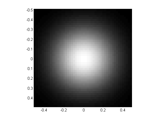
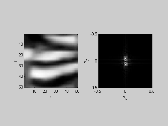
A really simple filter blurs an image using an impulse response as a Gaussian. That is, it turns points in to Gaussians. Let's create its impulse response:

wDeg = 1;  %size of image (in degrees)
nPix = 50;  %resolution of image (pixels);

[xf,yf] = meshgrid(linspace(-wDeg/2,wDeg/2,nPix+1));
xf = xf(1:end-1,1:end-1);
yf = yf(1:end-1,1:end-1);

sigma = .3;  %width of Gaussian (1/e half-width)
Gaussian = exp(-(xf.^2+yf.^2)/sigma^2);
figure(1)
clf
showImage(Gaussian,xf,yf);

The transformation of an image by this filter is done by convolution, just like the 1-D case. The 2-D convolution at any specific pixel location is calculated by placing the filter on the image centered on the pixel, multiplying the image values by their corresponding filter values and adding it all up (i.e. the dot product of the image and the filter). The whole image is filtered by doing this at every pixel location, effectively 'sliding' the filter around the image (like the 'smudge' tool in Photoshop).

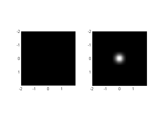
Matlab's 2-D function is 'conv2'. Let's convolve an image containing a single white pixel with the Gaussian:

wDeg = 4;  %size of image (in degrees)
nPix = 200;  %resolution of image (pixels);

[x,y] = meshgrid(linspace(-wDeg/2,wDeg/2,nPix+1));
x = x(1:end-1,1:end-1);
y = y(1:end-1,1:end-1);

img = zeros(size(x));
img(end/2,end/2) = 1;

filtImg = conv2(img,Gaussian,'same');

figure(1)
subplot(1,2,1)
showImage(img,x,y);
subplot(1,2,2)
showImage(filtImg,x,y);

% Not surprisingly, we get the impulse response back because we calculated
% the response to an impulse (duh).
%

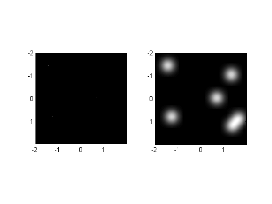
Superposition

Filtering the sum of two images is the same as adding the images after filtering. So a filtered image containing a few sparse pixels becomes a few Gaussians. The Gausisans add on top of eachother if the underlying pixels are close enough so they overlap.

img = zeros(size(x));
img(rand(size(img))>1-5/nPix^2) = 1;

filtImg = conv2(img,Gaussian,'same');

figure(1)
subplot(1,2,1)
showImage(img,x,y);
subplot(1,2,2)
showImage(filtImg,x,y);

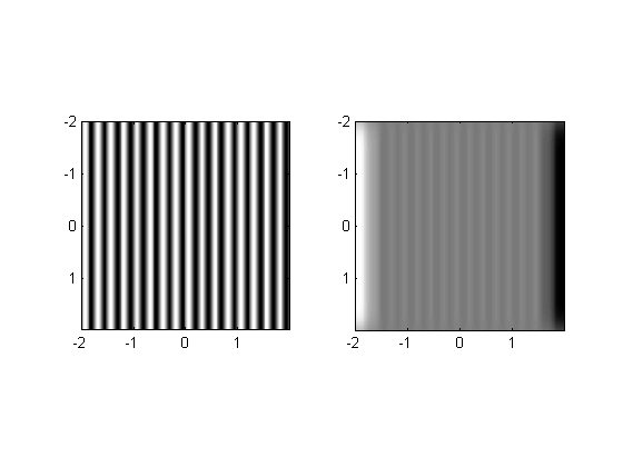
Filtering gratings

Just like for the 1-D case, when a grating is passed through a linear shift-invariant filter the output is a grating of the same spatial frequency. Only the amplitude and phase are changed. Here's what happens when you filter a grating with the Gaussian filter:

Make a grating;

orientation = 90;  %deg (counter-clockwise from horizontal)
sf = 4; %spatial frequency (cycles/deg)

ramp = sin(orientation*pi/180)*x-cos(orientation*pi/180)*y;

grating = sin(2*pi*sf*ramp);

filtImg = conv2(grating,Gaussian,'same');
plotResp2(grating,filtImg,x,y);

We'll always get a grating, no matter how weird our impulse response is:

weirdFilt = rand(size(Gaussian))-.5;

filtImg = conv2(grating,weirdFilt,'same');
plotResp2(grating,filtImg,x,y);

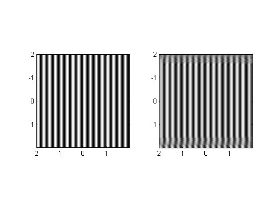
Except for the edge artifacts, notice how the inside of the image is a grating of the same frequency, and how the phase and amplitude changes.

So, like the 1-D case, we have the following facts:

1) Any 2-D image can be represented as a sum of gratings. 2) Linear filtering satisfies the properties of superposition and additivity. 3) A filtered grating is just another grating of the same frequency.

From these three facts, it follows that a filter can be completely described by how it transforms sinusoidal gratings. And, since the impulse response also completely describes the filter, the fft of the impulse response does too. This means that we can look at the fft of the impulse response to see what parts of the frequency spetrum pass through the filter.

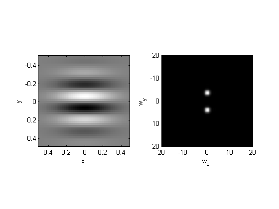
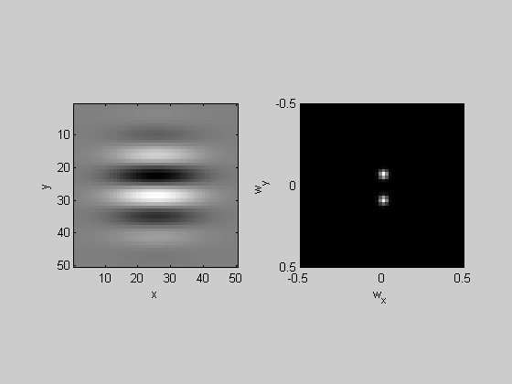
A good example is a Gabor filter:

orientation = 0;  %deg (counter-clockwise from horizontal)
sf =3.75; %spatial frequency (cycles/deg)

ramp = sin(orientation*pi/180)*xf-cos(orientation*pi/180)*yf;

grating = sin(2*pi*sf*ramp);
Gabor = grating.*Gaussian;
plotFFT2(Gabor,xf,yf,3,20);

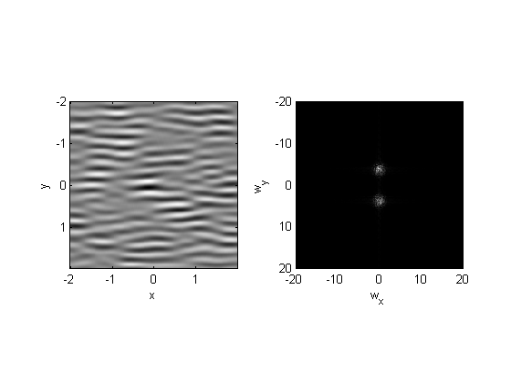
When we filter noise by the Gabor filter, we're only allowing through the grating components in the noise that correspond to the amplitudes in the filter:

noise = randn(size(x));

filtNoise = conv2(noise,Gabor,'same');
plotFFT2(filtNoise,x,y,3,20);

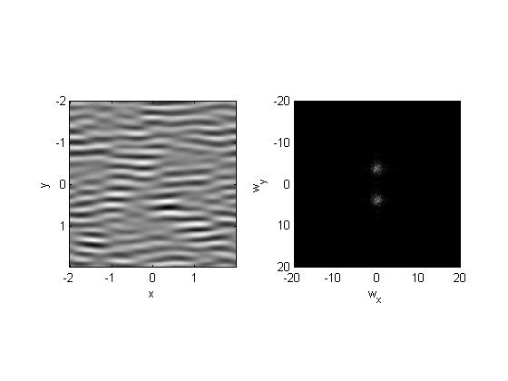
This should look familiar. In the previous lesson we did a similar thing by multiplying the amplitudes in the frequency domain. It should be clear, now, that there are two ways to filter an image - either through convolution of the impulse response function or by multiplying the fft of the image by the fft of the impulse response function.

To demonstrate, we'll do the same filtering in the frequency domain:

fftFilt = fft2(Gabor,size(x,1),size(x,2));
fftNoise = fft2(noise);
fftFiltNoise = fftFilt.*fftNoise;
filtNoise2 = ifft2(fftFiltNoise);

plotFFT2(filtNoise2,x,y,3,20);

Where's Waldo?

I've scanned in (without copyright permission) a page from a 'Where's Waldo' book. Let's build a filter to help find Waldo. First we'll read in the image and crop it to be square.

waldo = imread('Waldo.bmp');

%waldo = imread('TheGobblingGluttons.jpg');
%waldo = imread('DepartmentStore.jpg');

figure(1)
clf
image(waldo);
axis equal
axis tight

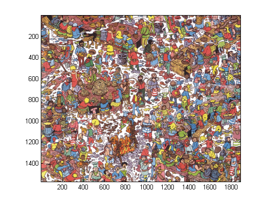
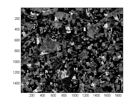
%Our goal is to build a filter that finds Waldo.  This will be done by
%analyzing a component of the image containing Waldo-like features.
%
%Since Waldo's stripes are red and white, how do we combine the r,g, and b
%images to make a grayscale image where the stripes are black and white?
%
%Our transformation will be: red - (.5*green + .5*blue)

waldo2D = double(waldo(:,:,1)-.5*waldo(:,:,2)-.5*waldo(:,:,3));
waldo2D = waldo2D-mean(waldo2D(:));

figure(1)
clf
imagesc(waldo2D)
colormap(gray);
axis equal
axis tight

%Let the user click on a possible location of 'Waldo' (e.g. stripes) and crop the
%image down to the region around where the mouse was clicked. Then show the
%cropped image in figure 2.
%
%The user input is done with 'ginput' which waits for the user to click the
%mouse on the current figure and returns the x and y positions.  the '1'
%means wait for just one click.

figure(1)
[xClick,yClick] = ginput(1);
xClick = round(xClick);
yClick = round(yClick);

%size of square patch (pixels)
sz = 50;

patch2D  = waldo2D(yClick-sz/2:yClick+sz/2-1,xClick-sz/2:xClick+sz/2-1);

Now we'll calculate the spatial freqency of the stripes.

[xx,yy] = meshgrid(linspace(-sz/2,sz/2,sz));
patch2D= patch2D-mean(patch2D(:));

figure(2)
clf
plotFFT2(patch2D);

Have the user click on the 2D fft to get the spatial frequency:

subplot(1,2,1);
[foo,sf] = ginput(1);

disp(sprintf('Spatial Frequency: %5.2f cycles/pixel',sf));

Spatial Frequency:  0.08 cycles/pixel

Make a sin-phase Gabor with the desired spatial frequency:

sigma = 1/sf;  %width of Gaussian (1/e half-width)
Gaussian = exp(-(xx.^2+yy.^2)/sigma^2);

gratingSin = sin(2*pi*sf*yy);
GaborSin = gratingSin.*Gaussian;

figure(2)
clf
plotFFT2(GaborSin);

Filter the image with 'GaborSin' and look at the result:

filtImgSin = conv2(waldo2D,GaborSin,'same');

figure(3)
clf
imagesc(filtImgSin);
axis equal
axis off
colormap(gray);

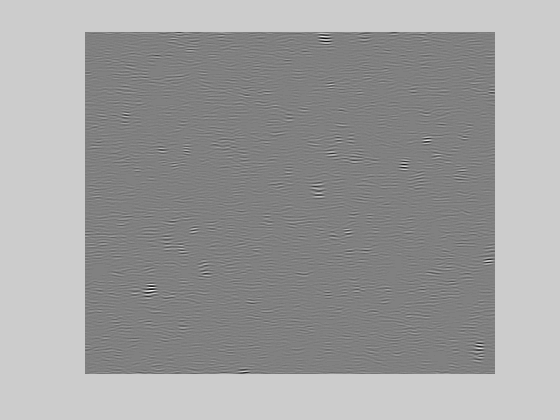
Notice that the filter does pick up on the locations in the Waldo image containing stripes, but the filtered image has stripes, too. This is because the output of filtering by our Gabor is dependent upon spatial phase. In the convolution process, when the filter and the image match up, the output is a large positive number, but when they're out of phase, the output is a large negative number.

Another way to think about it is to remember that a filtered sinusoid is also a sinusoid. So where the waldo image is sinusoidal, the filtered output will be sinusoidal too.

What we really want is a filtering process that picks up on the stripey parts, but doesn't depend on phase. One way to do this is to filter with Gabors of both sin and cosine phase and combine the outputs. Since sin^2+cos^2=1, it follows that the sum of squared outputs of the filtered images will only reflect the amplitude of the sinusoids in the image.

The two filters are called a 'quadrature pair'.

The next step convolves the image with a cosine-phase Gabor:

gratingCos = cos(2*pi*sf*yy);
GaborCos = gratingCos.*Gaussian;

filtImgCos = conv2(waldo2D,GaborCos,'same');

Our phase-invariant filtered image is combined by taking the square root of the sum of squares of the two phase-dependent filtered images.

filtImg = sqrt(filtImgSin.^2+filtImgCos.^2);

figure(3)
clf
imagesc(filtImg)
axis equal
axis off
colormap(gray);

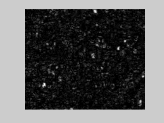
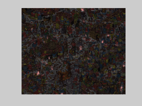
This next part modifies the original Waldo image by multiplying it point-by-point with a scaled version of our phase-invariant filtered image. It makes the image darker where there is red and white stripey stuff.

attenuateImg = filtImg/max(filtImg(:));
attenuateImg = (attenuateImg+.25)/1.25;

newImg = uint8(double(waldo).*repmat(attenuateImg,[1,1,3]));
figure(3)
clf

image(newImg);
axis equal
axis off

Exercises

1) Find some more Waldo images on the web and see if you can get the code above to find Waldo. Since the spatial frequencies of the images are in cycles/pixel, the code doesn't rely on an assumption about the image size, so it should generally work. You might have to mess with the size of the filter ('sz').

2) The Waldo image has a couple of green and white stripey distractors. Can you combine the image colors and run the code so that it finds these distractors instead?

3) What does the filter find when you use a zero spatial frequency filter (e.g. a Gaussian)?

Published with MATLAB® 7.6