Lesson 6: Introduction to the Bootstrap

When we summarize a data set with a statistic, such as when we calcualte a threshold from psychometric function data, we'd also like to know something about the reliability of that statistic. The brute-force way to estimate this reliability is to run the same experiment multiple times and calculate the mean and standard error of our statistic. But this can be time-consuming and expensive. Fortunately, there is a way of estimating the variability of a statistic from a single data set. This 'bootstrapping' method seems like magic, but as we'll demonstrate here it works remarkably well.

Contents

The mean as a simple example of a statistic

The arithmetic mean is used so commonly that we don't really think of it as one particular way to summarize a list of numbers - that is, as a 'statistic'. But if you think about it, it's one of many ways to estimate the 'central tendency' of a data set (e.g. there's also the median and mode). Since the mean is used so commonly, we have a firm understanding about how it behaves for different set sizes. Specfically, we have the Central Limit Theorem that states that for sufficiently large data sets, the mean will be distributed normally and will have a standard deviation that shrinks by a factor of 1/sqrt(n) where n is the size of the data set.

We can demonstrate this in Matlab in just a couple of lines of code. We'll generate 25 numbers 2000 times from a unit normal distribution (mean 0, variance 1) and look at the distribution of the 2000 means:

clear all

First we'll do something a little weird. We're using the statistic 'mean' as an example, but I want to be able use other functions as well. This is a perfect time to introduce the 'function handle', which is a way of defining a variable that acts as a function. We can then later change the definition of this variable so that a different calculation is made every time this variable is 'used'.

We'll define the function handle 'myStatistic' to be the function 'mean'

myStatistic = @mean;

% Here's an option for an arbitrary statistic (commented out)
% myStatistic = @(x) abs(mean(x))

Now we'll run our statistic on 2000 sample data sets, each with 25 numbers drawn from a unit normal.

n = 25;  %size of each data set
nReps = 2000;  %number of data sets or 'experiments'

data = randn(n,nReps);  %n x nReps draws from unit normal probability distribution

populationStat = zeros(1,nReps);
for i=1:nReps
    %Calculate our statistic on each column in 'data'
    populationStat(i) = myStatistic(data(:,i));
end

If our statistic is the mean, then we'll show that the standard deviation 'populationStat' is close to 1/sqrt(n) = 1/5 = 0.2;

if strcmp(func2str(myStatistic),'mean')
    disp(sprintf('Expected s.d.: %g, Actual s.d.: %5.3f',1/sqrt(n),std(populationStat)));
end

Expected s.d.: 0.2, Actual s.d.: 0.199

We'll show the distribution of our statistic as a histogram:

figure(1)
clf
hist(populationStat,50)  %50 bins
xlabel(func2str(myStatistic));
title('Samples drawn from the population');

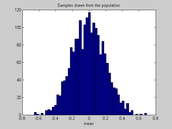
Instead of using the standard deviation as a measure of variability, from here on we'll talk about 'confidence intervals'. This is a better way of describing variability when dealing with non-normal distributions. A 95% confidence interval contains the middle 95% of the numbers in a list. The confidence interval associated with the standard deviation is roughly the 68% confidence interval, since interval between -1 and 1 under the unit normal distribution contains about 68% of the area.

A more precise value of the percent for 1 standard deviation can be calculated with the 'Cumulative Normal' function, which gives the area under the normal distribution to the left of x:

CIrange = 100*(NormalCumulative(1,0,1) - NormalCumulative(-1,0,1));
%
% For our example, this confidence interval of about 68% should be between
% -.2 and 0.2, since 0.2 is the expected standard deviation.

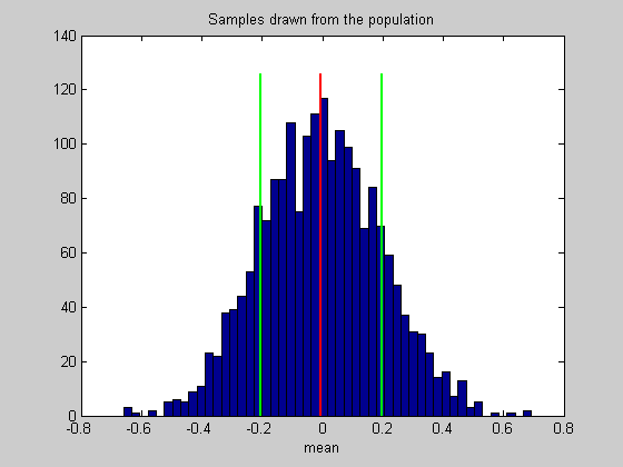
The endpoints of the confidence interval can be calcualted with Matlab's 'prctile' function.

populationCI = prctile(populationStat,[50-CIrange/2,50+CIrange/2]);

Draw the mean and confidence interval on the histogram

hold on
ylim = get(gca,'YLim');

plot(mean(populationStat)*[1,1],ylim*1.05,'r-','LineWidth',2);
plot(populationCI(1)*[1,1],ylim*1.05,'g-','LineWidth',2);
plot(populationCI(2)*[1,1],ylim*1.05,'g-','LineWidth',2);

Bootstrapping from a single data set

Suppose we only have one data set of 25 numbers and don't have the luxury of running the experiment 2000 times. So we only have a single calculation of our statistic form this one 'experiment':

x = randn(1,n);
sampleStat = myStatistic(x);

Sampling with replacement

How can we estimate the variability of this statistic from just this information? The trick is to run a simulation much like we did before, but instead of drawing 25 numbers from the population, we draw 25 numbers 'with replacement' from our existing set of 25 numbers. 'Sampling with replacement' means to draw numbers out of the 25 while allowing for repeated draws of the same number.

Sampling with replacement is easy in Matlab. First we generate a matrix of integers that range from 1 to n to use as indices into our existing data set.

id = ceil(rand(n,nReps)*n);

Then we use this index to 'sample' our existing data set:

bootstrapData = x(id);

Finally, we'll calculate our statistic on each of the columns containing 25 draws.

bootstrapStat = zeros(1,nReps);
for i=1:nReps
    bootstrapStat(i) = myStatistic(bootstrapData(:,i));
end

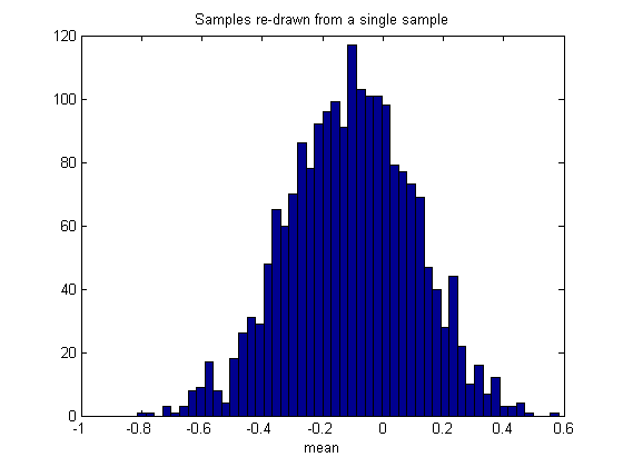
We'll show the distribution of our bootstrapped statistic as a histogram:

figure(2)
clf
hist(bootstrapStat,50)  %50 bins
xlabel(func2str(myStatistic))
title('Samples re-drawn from a single sample');

Then calculate and draw the confidence intervals like we did before

bootstrapCI = prctile(bootstrapStat,[50-CIrange/2,50+CIrange/2]);

hold on
ylim = get(gca,'YLim');
h1=plot(bootstrapCI(1)*[1,1],ylim*1.05,'g-','LineWidth',2);
plot(bootstrapCI(2)*[1,1],ylim*1.05,'g-','LineWidth',2);

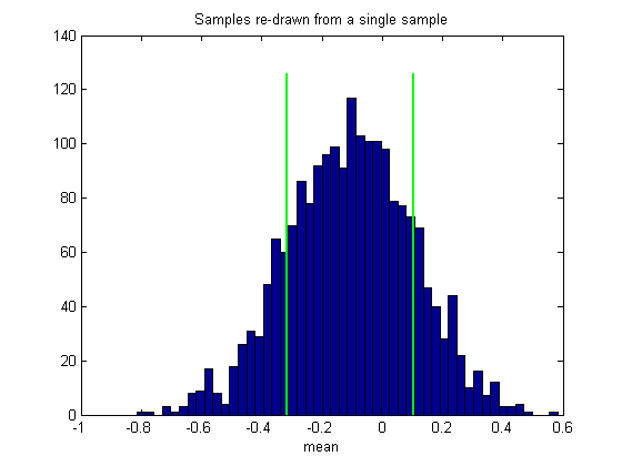
Notice that the mean of our bootstrapped statistic isn't zero. In fact, the mean of this histogram should be very near the statistic on the sample we used to generate the boostsrap, which we'll mark on the histogram:

plot(sampleStat*[1,1],ylim*1.05,'r-','LineWidth',2);

This illustrates an important point about the bootstrap method: The distribution of bootstrapped statistics won't necessarily match the distribution of the statistics on the population (compare figures 1 and 2), even if we could increase our number of bootstrapped measures to infinity.

The'bias-corrected and accelerated' (BCa) confidence interval

There's one more step in the way the confidence intervals are calculated in practice. It turns out that there's a slight bias in this basic procedure which is most apparent when the distribution of the statistic is skewed.

On average, the boostrap confidence interval will be slightly too narrow. If the statistic is 'mean', then in the limit the width of the confidence interval is exactly what you'd expect if you used the 'population' standard deviation instead of the 'sample' standard deviation for the expected width. That is, if the standard devaiation function used when calculating the expected width used an 'n' in the denominator instead of 'n-1'.

I've implemented this BCa method, along with the general bootstrapping procedure we used above in a single a function called 'bootstrap'. It takes in as arguments a handle to our statistic, the sample values (which we call x), the number of repetitions and a confidence interval range. Here's how to use it:

bootstrapCI = bootstrap(myStatistic,x,nReps,CIrange);

For comparison we'll plot this 'corrected' confidence interval on the histogram:

h2=plot(bootstrapCI(1)*[1,1],ylim*1.05,'y-','LineWidth',2);
plot(bootstrapCI(2)*[1,1],ylim*1.05,'y-','LineWidth',2);

legend([h1,h2],{'original','corrected'});

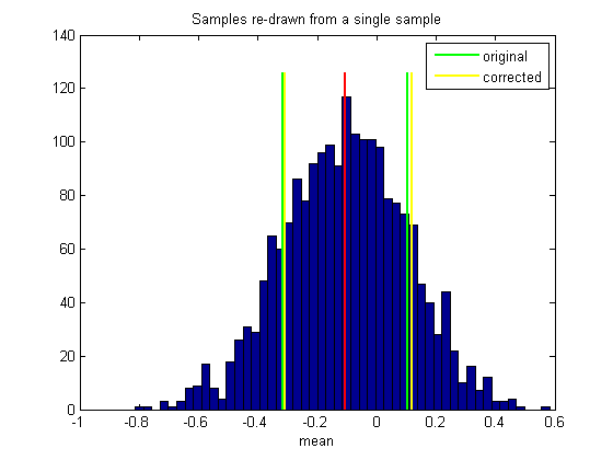
For our well-behaved function 'mean' the two confidence intervals will be very similar. So for this example, this complicated correction procedure doesn't make much difference. If you understand the basic bootstrap method (without correction), you have about 99% of the intuition for the whole procedure.

Hypothesis testing

The bootstrapping algorithm tells us something about the reliability of our statistic based on our simple sample. We can use the confidence interval to test the hypothesis that the statistic run on our sample of 25 numbers is significantly difference from the population average.

In the real world, we don't know the population average (that's what we're trying to estimate), but in our simulation the population average will be close to the mean of the distribution show in figure 1, since this is the distribution of 2000 statistics based on the population.

nullStat = mean(populationStat);  %null hypothesis statistic

It'll be pretty close to zero for the statistic 'mean'

For hypothesis testing, we'll use the ubiquitious '.05' criterion level (95% confidence interval)

CIrange = 95;
bootstrapCI = bootstrap(myStatistic,x,nReps,CIrange);

Here are the locations of the endpoints for the 95% confidence interval:

plot(bootstrapCI(1)*[1,1],ylim*1.05,'k-','LineWidth',2);
plot(bootstrapCI(2)*[1,1],ylim*1.05,'k-','LineWidth',2);

%Is the population mean 'nullStat' outside our confidence interval?  Let's
%find out:
if nullStat<bootstrapCI(1) || nullStat>bootstrapCI(2)
    str = 'Reject';
else
    str = 'Fail to reject';
end
disp(sprintf('%s the null hypothes at alpha = %5.2f',str,(1-CIrange/100)));

Fail to reject the null hypothes at alpha =  0.05

By design, we should reject the null hypothesis 5% of the time. These 5% are 'Type I' errors because the sample was drawn from the population so we know that the null hypothesis is true.

To check this, we'll run 1000 'Experiments' where in each experiment we do what we just did: generate a sample data set, calculate the statistic and 95% confidence intervals and run the hypothesis test.

This takes a little while - each experiment calls 'bootstrap' which in turn runs 2000 statistics on resampled data. We'll use matlab's 'waitbar' to track the progress so we know whether or not we have time to go get a cup of coffee.

nExperiments = 1000;
CIrange = 95;
nReject = 0; %this will be incremented every time the null hypothesis is rejected

set up the 'waitbar'

h = waitbar(0,sprintf('running %d "experiments"',nExperiments));

for i=1:nExperiments
    %pull out a new sample
    x = randn(1,n);
    CI = bootstrap(myStatistic,x,nReps,CIrange,1);
    if nullStat<CI(1) || nullStat>CI(2)
        nReject = nReject+1;
    end
    waitbar(i/nExperiments,h)
end

delete(h)

disp(sprintf('Rejection of null hypothesis: Expected: %5.3f, Simulated: %5.3f',(1-CIrange/100),nReject/nExperiments));

Rejection of null hypothesis: Expected: 0.050, Simulated: 0.073

This is a little scary. I consistently find that I reject the null hypothesis more often than I should - even with a simple statistic like 'mean'. This means that the bootstrapping algorithm might be leading people to claim positive results when they're really not significant. Yikes!

Comparing our 'bootstrap' function to Matlab's 'bootc'

Matlab provides a bootstrapping function that does essentially the same thing as 'bootstrap'; that is it can calculate the confidence interval using the 'bias accelerated' correction (it can do other things too). If you have purchased Matlab's statistic toolbox you can run the next section to compare matlab's version with ours. If not, the punchline is that the two programs give essentially the same answer. Interestingly, since the bootstrap is a stochastic process, neither method gives the same answer every time. But it looks like the distribution of answers from both programs are identical, meaning that the two functions are doing the same thing.

nExperiments = 	1000;
ours = zeros(nExperiments,2);
theirs = zeros(nExperiments,2);

h = waitbar(0,sprintf('running %d simulations',nExperiments));
for i=1:nExperiments
    ours(i,:)  = bootstrap(myStatistic,x,nReps,CIrange,1)';
    theirs(i,:) = bootci(2000,{myStatistic, x}) ;
    waitbar(i/nExperiments,h)
end

delete(h)

Plot histograms of our 'bootstrap' interval endpoints along with those from 'bootci'

figure(3)
clf

for i=1:2
    subplot(1,2,i)
    hist([ours(:,i),theirs(:,i)])
    if i==1
        title('Low')
    else
        title('High')
    end
    disp(sprintf('Means: ours %g, theirs %g',mean(ours(:,i)),mean(theirs(:,i))));
    disp(sprintf('S.D.: ours %g, theirs %g',std(ours(:,i)),std(theirs(:,i))));
end

Means: ours -0.294514, theirs -0.293777
S.D.: ours 0.0145232, theirs 0.0142229
Means: ours 0.601682, theirs 0.601807
S.D.: ours 0.0216003, theirs 0.0212208

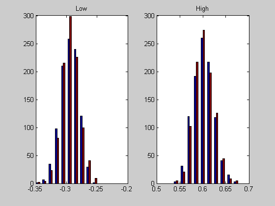
Since matlab's 'bootci' and our 'bootstrap' appear to be the same, our scary observation that we're rejecting the null hypothesis too often remains scary (or gets scarier).

Exersises

Published with MATLAB® 7.6