Lesson 7: Using the bootstap to estimate variability in thresholds

Now that we've introduced the bootstrapping procedure for a general function, we're ready to apply it to estimating the variability in the threshold parameter from the best-fitting Weibull function.

Contents

The procedure is similar, but not the same as the previous lesson so we won't be able to use our 'bootstrap.m' function. The main difference is that we'll be using a 'parametric' bootstrap in stead of the 'non-parametric' bootstrap that we used earlier. By 'parametric', we mean that the 'fake' data sets will be generated usinga binary process based on the best-fitting Weibull function, not by resampling the actual psychophysical data.

We'll use the parametric procedure mainly because it has been suggested in a paper by Wichmann and Hill (Perception and Psychophysics, 2001). They make two compelling arguments for the parametric method: (1) by assuming that a Weibull function generated our orignal data set, we've already committed to a parametric function anyway and we're making no further assumptions with the boostrap and (2) the raw data is presumably the result of a binary process, so it doesn't make sense to treat these raw values as measurements of the exact mechanism that lead to their values. Rather, it makes more sense to employ a similar binary process to generate the 'fake' data sets in the resampling process.

As in the last lesson we'll go through step-by-step the main procedure, which gets us through 90% of the work (and about 100% of the intuition). The final step - the 'bias corrected accellerated' method for calculating the confidence intervals has been incorporated into a function that I've provided and won't be discussed in detail. For details, view the function and see Efron and Tibshirani's "Introduction to the Bootsrap" (Chapman & Hall/CRC, 1993, pages 178-201)

We'll use our staircase data from the previous lesson as our test data set:

clear all
load resultsStaircase

First, we'll calculate the threshold by fitting the Weibull function to the data, just as we did before:

Initial parameters:

pInit.t = .1;
pInit.b = 2;
pInit.shutup = 1;
freeList ={'t','b'};

Call the 'fit' function

[pBest,logLikelihoodBest] = fit('fitPsychometricFunction',pInit,freeList,results,'Weibull');

Save the threshold for later.

thresh = pBest.t;

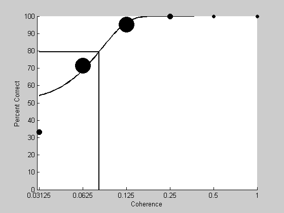
Here's a plot the psychometric function (again) and the best-fitting Weibull in black

intensities = unique(results.intensity);

nCorrect = zeros(1,length(intensities));
nTrials = zeros(1,length(intensities));

for i=1:length(intensities)
    id = results.intensity == intensities(i) & isreal(results.response);
    nTrials(i) = sum(id);
    nCorrect(i) = sum(results.response(id));
end

pCorrect = nCorrect./nTrials;

figure(1)
clf
hold on

%loop through each intensity so each data point can have it's own size.
for i=1:length(intensities);
    sz = nTrials(i)+2;
    plot(log(intensities(i)),100*pCorrect(i),'ko','MarkerFaceColor','k','MarkerSize',sz);
end

%plot the parametric psychometric function
x = exp(linspace(log(min(results.intensity)),log(max(results.intensity)),101));
y = Weibull(pBest,x);

plot(log(x),100*y,'k-','LineWidth',2);
plot([log(min(x)),log(pBest.t),log(pBest.t)],[100*(1/2)^(1/3),100*(1/2)^(1/3),0],'k-','LineWidth',2)

set(gca,'XTick',log(intensities));
logx2raw
set(gca,'YLim',[0,100]);
xlabel('Coherence');
ylabel('Percent Correct');

The parametric bootstrap

Next we'll repeatedly generate 'fake' data sets based on this best-fitting Weibull function. Each new binary 'response' will be based on a coin flip biased by the Weibull's probability for the associated stimulus intensity.

Bootstrapping usually involves many resamples of the original data, but before we do this it's instructive to run just a few and look at the resulting psychometric functions and fits.

nReps = 5;               %just a few
colList = hsv(nReps+1);  %list of colors for plotting

Evaluate the Weibull at the stimulus intensity values using the best-fitting parameters

prob = Weibull(pBest,results.intensity);

'bootResults' will contain each 'fake' data set

bootResults.intensity = results.intensity;

for repNum=1:nReps
    % generate the 'fake' responses using coin flip biased by 'prob'
    bootResults.response = floor(rand(size(results.response))+prob);
    % fit 'bootResults' with the Weibull - use pBest as initial values
    [pBoot,logLikelihoodBest] = fit('fitPsychometricFunction',pBest,freeList,bootResults,'Weibull');

    % plot the results like we just did for the real data
    for i=1:length(intensities)
        id = bootResults.intensity == intensities(i) & isreal(bootResults.response);
        nTrials(i) = sum(id);
        nCorrect(i) = sum(bootResults.response(id));
    end

    pCorrect = nCorrect./nTrials;

    %loop through each intensity so each data point can have it's own size.
    for i=1:length(intensities);
        sz = nTrials(i)+2;
        plot(log(intensities(i)),100*pCorrect(i),'ko','MarkerFaceColor',colList(repNum,:),'MarkerSize',sz);
    end

    %plot the best-fitting Weibull function and lines depicting the threshold
    x = exp(linspace(log(min(results.intensity)),log(max(results.intensity)),101));
    y = Weibull(pBoot,x);

    plot(log(x),100*y,'k-','Color',colList(repNum,:));
    plot([log(min(x)),log(pBoot.t),log(pBoot.t)],[100*(1/2)^(1/3),100*(1/2)^(1/3),0],'k-','Color',colList(repNum,:))
end

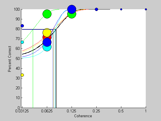
It's interesting to see how much variability there is in the psychometric functions even though they were all generated by the same Weibull parameters. This shows how even without any inherent variability in the subject's threshold, the resulting psychometric function will still have a remarkable amount of variability which will lead to variability in the estimated threshold. This variability, or 'noise' is inherent in the binary process, and can be thought of as a lower bound for the noise in the threshold measurement. Other sources of noise, like session-to-session drifts in the actual shape of the subject's internal Weibull function will only add to this variability.

We'll now run the parametric boostrap on many, many more repetitions. A common number is 2000, which takes about 5 minutes on my laptop. We'll use the 'waitbar' to track the computer's progress.

nReps = 2000;  %2000 is a typical number - it takes about 5 minutes on my laptop.

'bootResults' will hold our 'fake' data set

bootResults.intensity = results.intensity;

Zero out some parameters and start the loop.

bootThresh =zeros(1,nReps);

% set up the 'waitbar'
h = waitbar(0,sprintf('Bootstrapping %d fits',nReps));
for i=1:nReps
    % generate the 'fake' responses using coin flip biased by 'prob'
    bootResults.response = floor(rand(size(results.response))+prob);
    % fit the 'fake' data with the Weibull - use pBest as initial values
    [pBoot,logLikelihoodBest] = fit('fitPsychometricFunction',pBest,freeList,bootResults,'Weibull');
    % save the threshold for this iteration
    bootThresh(i) = pBoot.t;
    % update the 'waitbar'
    waitbar(i/nReps,h)
end
%remove the waitbar
delete(h)

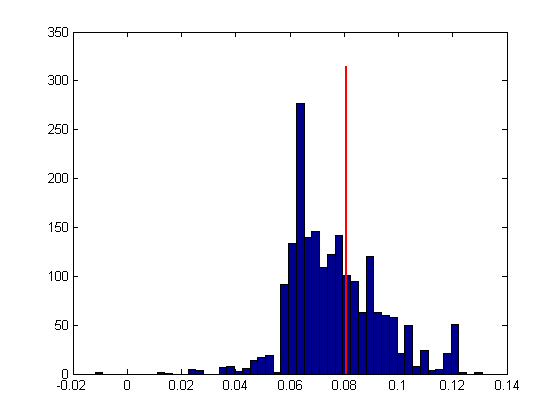
We now have a distribution of thresholds. Let's take a look at this ditribution as a histogram, along with the actual threshold:

figure(2)
clf
hist(bootThresh,50);
hold on
ylim = get(gca,'YLim');
plot(thresh*[1,1],ylim*1.05,'r-','LineWidth',2)

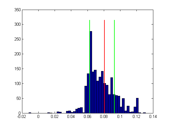
As with the non-parametric bootstrap, we'll calculate the 68% confidence interval (68% corresponds to +/- 1 standard deviation for a normal distribution, so it's like a general standard error of the mean).

CIrange = 68.27;

CI = [prctile(bootThresh,(100-CIrange)/2),prctile(bootThresh,(100+CIrange)/2)];

plot(CI(1)*[1,1],ylim*1.05,'g-','LineWidth',2)
plot(CI(2)*[1,1],ylim*1.05,'g-','LineWidth',2)

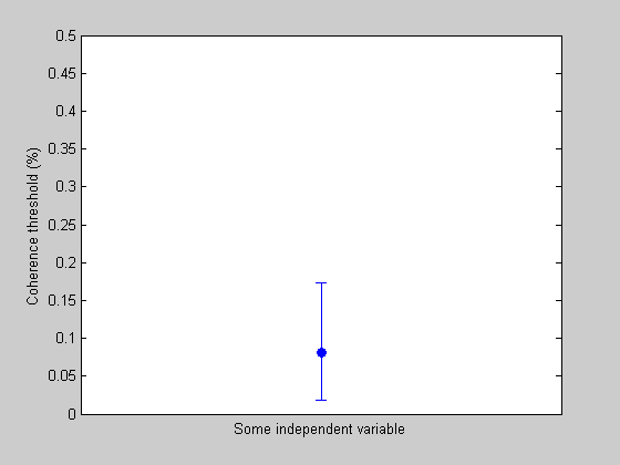
Plotting with an errorbar

We have a threshold with an errorbar, which we can plot (it'll look stupid by itself, but it shows how to use 'errorbar').

figure(3)
clf
plot(1,thresh,'o','MarkerFaceColor','b');
hold on
errorbar(1,thresh,CI(1),CI(2));
set(gca,'XLim',[0.5,1.5]);
set(gca,'YLim',[0,.5]);
ylabel('Coherence threshold (%)');
xlabel('Some independent variable');
set(gca,'XTick',[-nan,nan]);

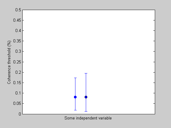
The function 'bootstrapWeibullThreshold'

This is basically it. The only thing missing is the correction for a bias and skew in the histogram using the 'bias corrected and accelerated (BCa) method. I've implemeted this method for the parametric bootstrap in the function 'bootstrapWeibullThreshold'. Here's how to use it.

[CI,thresh] = bootstrapWeibullThreshold(results,pInit,nReps,CIrange);

Plot the data point with the corrected errorbar next to the old one.

plot(1.1,thresh,'ko-','MarkerFaceColor','b');
hold on
errorbar(1.1,thresh,CI(1),CI(2));

set(gca,'YLim',[0,.5]);
set(gca,'XLim',[0.5,1.75]);

Exercises

Published with MATLAB® 7.6