Lesson 8: Signal Detection Theory and the 'yes/no' experiment

A fundamental theory that can predict a variety of basic detection and discrimination task is 'Signal Detection Theory', or SDT for short. This lesson defines some of the basic principles of SDT and shows how to calculate it from a single 'yes/no' detection experiment.

Contents

The simple 'yes/no' forced choice experiment

Before getting to the 2AFC experiment, we'll start with a simpler version where either no stimulus or a weak stimulus is presented on each trial and the subject must respond 'yes' or 'no' to indicate whether or not anything was seen. The classic example is a very dim flash of light in the dark.

The idea behind SDT is that there is 'noise' in the system that interferes with perfect performance on the task. The noise can either be external, caused by variability in the number of photons in the flash, for example or internal, caused by intrinsic variablity in the neuronal representation of the stimulus. This means that the internal response to any stimulus will vary from trial to trial. Sometimes the noise in a trial containing no stimulus (a 'noise' trial) will produce a large enough response that the subject will claim to see a stimulus, causing a false alarm. Or, sometimes a trial containing a stimulus (a 'signal trial) will lead to a weak response, causing the subject to respond 'no' - a 'miss' trial.

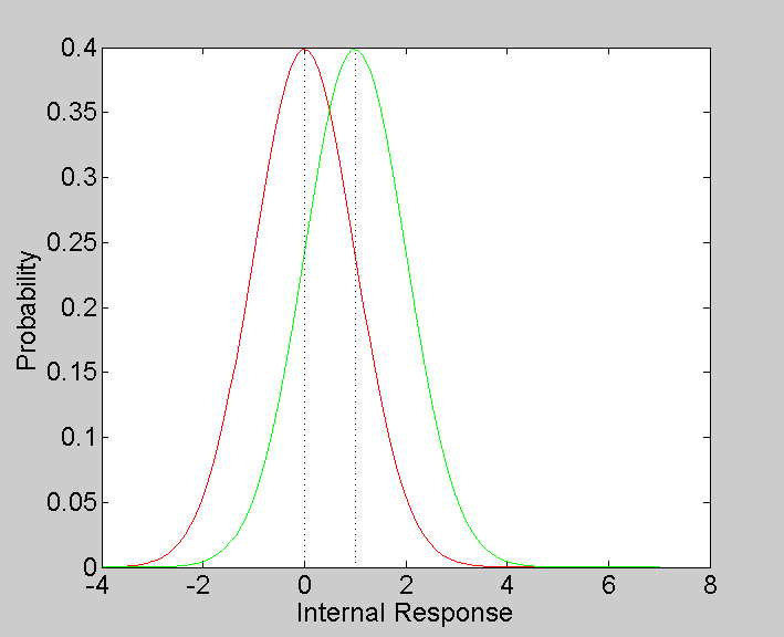
Formally, the internal representation is along a single dimension, and the response to a given stimulus is described by a probability distribution function (PDF) along that dimension. In the simplest case, 'noise' and 'signal' trial distributions will be normally distributed with equal variances but different means.

Let's choose some numbers and draw the PDF's for illustration. To keep things simple, we'll choose a variance of 1, so that our normal distributions will be 'unit normals'.

clear all

variance = 1;

noiseMean = 0;
signalMean = 1;

x = linspace(-4,7,101);  %x-axis values

The PsychToolbox provides us with a function 'NormalPDF' which is simply a Gaussian function normalized so that its total area under the curve is 1.

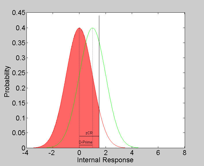
noisePDF = NormalPDF(x,noiseMean,variance);
signalPDF = NormalPDF(x,signalMean,variance);

figure(1)
clf
plot(x,noisePDF,'r')
hold on
plot(x,signalPDF,'g')
xlabel('Internal Response')
ylabel('Probability')

ylim = get(gca,'YLim');
plot(noiseMean*[1,1],ylim,'k:');
plot(signalMean*[1,1],ylim,'k:');

SDT is based on the idea that a subject chooses a 'criterion' level of internal response so that the decision on any trial is 'yes' if the internal response exceeds this criterion.

Criteria can range from being very conservative to avoid making misses, to being liberal to avoid making false alarms. The nature of the decision can influence this criterion. For example, a doctor reading an MRI might set a low criterion for detecting a tumor because the cost of missing a tumor is high compared to the cost of a false alarm. A subject sitting in the dark trying to see flashes of light, on the other hand, might not care so much about misses. This subject might set their criterion high and therefore only respond 'yes' when there is a very large internal response.

Let's set our criterion to a value of 1.5, and draw it on our graph

criterion = 1.5;

ylim = get(gca,'YLim');
plot(criterion*[1,1],[0,ylim(2)*1.1],'k-');

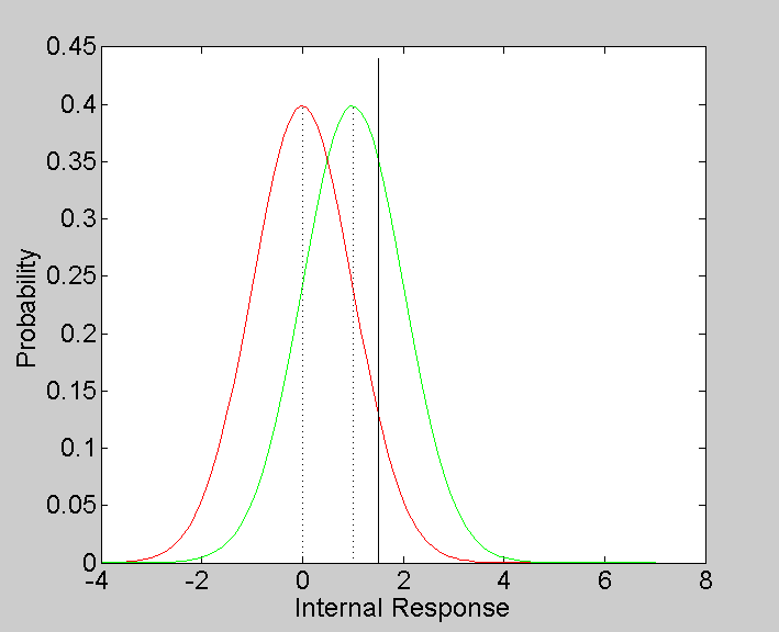
You can see from the graph that with this criterion, most trials will lead to a 'no' response because the bulk of both PDF's are below the criteron.

Definition of D-Prime

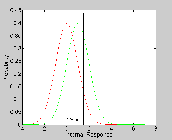
'Psychophysics' is the study of the relationship between physical stimuli and their psychological response. In the simple case for SDT with normal PDFs and equal variance, the strength of the psychological response, called 'D-Prime', is defined as the difference between the means of the signal and noise distributions normalized by the variance. With the noise mean set to zero (as it is in our example), D-Prime is the signal mean divided by its standard deviation:

dPrime = (signalMean-noiseMean)/variance

dPrime =

     1

plot([noiseMean,signalMean],[.01,.01],'k-');
text((noiseMean+signalMean)/2,.02,'D-Prime','HorizontalAlignment','Center');

The goal for the psychophysicist is to estimate D-Prime by having subjects view stimuli and make decisions - the ultimate goal is to provide an unbiased estimate of D-Prime with the minimal number of trials.

Estimating D-Prime from simple forced-choice

D-Prime can be estimated using a simple forced-choice method by assuming Signal Detection Theory with a fixed criterion. The goal is present both signal and noise trials and calculate the proportion of hits and 'correct rejections'.

This can be demonstrated through a simulation.

Here we'll simulate this subject's performance on a simple forced-choice task by randomly drawing from the normal distributions for a series of trials. This will use Matlab's 'randn' function.

nTrials = 100;

%Choose a random sequence of 'signal' and noise' trials with equal numbers:
stim = Shuffle(floor(linspace(.5,1.5,nTrials)));  %think about it...

resp = zeros(1,nTrials);
for i=1:nTrials
    if stim(i) == 0  %noise trial
        internalResponse = randn(1)*sqrt(variance)+noiseMean;
    else %signal trial
        internalResponse = randn(1)*sqrt(variance)+signalMean;
    end

    %Decision:
    resp(i) = internalResponse>criterion;
end

D-Prime can be calculated by looking at the performance for both the 'signal' and the 'noise' trials. Let's look at the noise trials first.

A 'correct rejection' is when the subject correctly responded 'no' on a noise trial. The proportion of correct rejections is therefore the number of times that resp and 'stim' are both zero divided by the total number of 'noise' trials:

pCR = sum(resp==0 & stim ==0)/sum(stim ==0)

pCR =

    0.9000

Looking at the figure, the proportion of correct rejections should be the area under the red curve to the left of the criterion. The criterion (in normalized units) can therefore be estimated by the z-score associated with the proportion of correct rejections.

Z-scores are calculated using the inverse of the normal CDF which (for some reason) is not provided in the PsychToolbox. I've written one myself using matlab's 'erfinv' function called 'inverseNormalCDF'

help inverseNormalCDF

 z = inverseNormalCDF(p)
 
 Calculates the inverse of the unit normal cumulative density function. 
 It returns the z-score corresponding to p, the area under the curve to the
 left in the unit normal distribution.  (See also Matlab's erfinv function)

zCR = inverseNormalCDF(pCR)

zCR =

    1.2816

plot([noiseMean,criterion],.04*[1,1],'k-')
text((noiseMean+criterion)/2,.05,'zCR','HorizontalAlignment','Center');

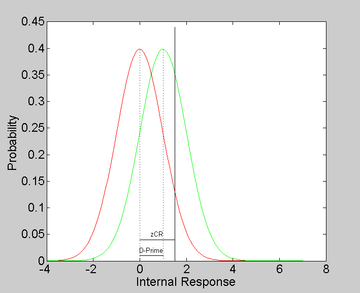
Note that the value of zCR should be close to the criterion we used to run the simulation.

We can color in this region this on the figure as a 'patch'

patchX = [linspace(-4,criterion,50),criterion,0];
patchY = [NormalPDF(linspace(-4,criterion,50),noiseMean,variance),0,0];
patch(patchX,patchY,'r','FaceAlpha',.6);

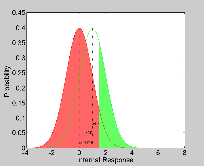
Now for 'signal' trials: The proportion of 'hits' is the number of trials where both 'resp' and 'stim' are equal to 1 divided by the total number of trials:

pHit = sum(resp==1 & stim==1)/sum(stim==1)

pHit =

    0.3400

plot([signalMean,criterion],.07*[1,1],'k-')
text((signalMean+criterion)/2,.08,'-zHit','HorizontalAlignment','Center');

This is equal to the area of green curve to the right of the criterion, which we can also fill in with a 'patch':

patchX = [linspace(criterion,8,50),criterion,criterion];
patchY = [NormalPDF(linspace(criterion,8,50),signalMean,variance),0,0];
h=patch(patchX,patchY,'g','FaceAlpha',.6);
%
% The z-score for the proportion of hits is the difference between the
% criterion and the mean of the signal trials.

zHit = inverseNormalCDF(pHit)

zHit =

   -0.4125

It follows that an estimate of d-prime is the sum of zCR and zHit:

dPrimeEst = zCR+zHit

dPrimeEst =

    0.8691

Is this close to the expected value?

This shows that in theory we can estimate D-Prime from a simple yes/no experiment. But as you might have noticed, even with 100 trials our estimate of D-Prime can be pretty far off from the expected value.

In many experiments, rather than finding D-Prime for a given condition, the experimenter wants to find the signal strength that produces a desired value of D-Prime (say dPrime = 1). So D-Prime must be measured across a range of stimulus strengths. You can imagine how difficult this must be to do with the yes/no method if estimating D-Prime at one stimulus strength is so variable.

Exercises

Published with MATLAB® 7.6