Lesson 9: ROC analysis

You can't discuss Signal Detection Theory without talking about the ROC, or 'Receiver Operating Characteristic' curve. In this lession we'll simulate subject's performance on a simple yes/no task for a range of criterion values to generate an ROC curve. We'll then compare the area under this curve to the results from a simulated 2AFC task.

Contents

Estimating D-Prime for a range of criterion values

D-Prime is a measure of the difference between the means for the signal and noise (in standard deviation units) so it shouldn't depend on the criterion. A classic test of signal detection theory in the behavioral sciences is to manipulate the subject's criterion across blocks of trials. This can be done in a variety of ways, including changing the rewards associated with hits and correct rejections.

Let's try this by simulating a bunch of yes/no trials across a range of criterion values. We'll use the same simulation method as we did in the previous lesson.

% Define the signal and noise distribution parameters:
variance = 1;

noiseMean = 0;
signalMean = 1;

% List of criterion values
criterionList = -4:.2:6;

% Number of trials for each criterion value
nTrials = 100;

% Zero out some vectors ahead of time
pCR = zeros(1,length(criterionList));
pHit = zeros(1,length(criterionList));
dPrimeEst = zeros(1,length(criterionList));

% Loop through the list of criterion values
for criterionNum = 1:length(criterionList)
    criterion = criterionList(criterionNum);

    %Choose a random sequence of 'signal' and noise' trials with equal
    %numbers:
    stim = Shuffle(floor(linspace(.5,1.5,nTrials)));  %think about it...

    resp = zeros(1,nTrials);
    for i=1:nTrials
        if stim(i) == 0  %noise trial
            internalResponse = randn(1)*sqrt(variance)+noiseMean;
        else
            internalResponse = randn(1)*sqrt(variance)+signalMean;
        end

        %Decision:
        resp(i) = internalResponse>criterion;
    end

    %Calculate our estimate of D-Prime, and save the correct rejection rate
    %and the hit rate for later.

    %Correct rejections
    pCR(criterionNum)  = sum(resp==0 & stim ==0)/sum(stim ==0);
    zCR = inverseNormalCDF(pCR(criterionNum) );

    %Hits
    pHit(criterionNum)  = sum(resp==1 & stim==1)/sum(stim==1);
    zHit = inverseNormalCDF(pHit(criterionNum) );

    dPrimeEst(criterionNum) = zCR+zHit;
end

Now we'll plot the estimated values of D-Prime on the y-axis with the criterion value on the x-axis

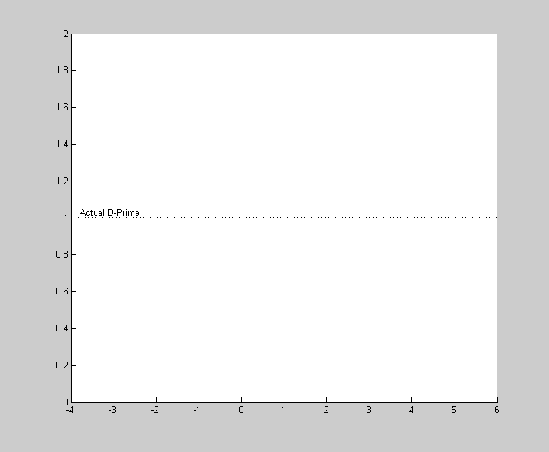
First we'll calculate the actual value of D-Prime from our parameters

dPrime = (signalMean-noiseMean)/sqrt(variance);

and plot this value as a horizontal dashed line, with some text to define it.

figure(1)
clf
hold on
plot([min(criterionList),max(criterionList)],dPrime*[1,1],'k:','LineWidth',2)
text(criterionList(2),dPrime,'Actual D-Prime','VerticalAlignment','Bottom');

Then we'll plot the estimated values of D-Prime on the same plot.

plot(criterionList,dPrimeEst,'ko','MarkerFaceColor','b')

xlabel('Criterion');
ylabel('Estimated D-Prime');

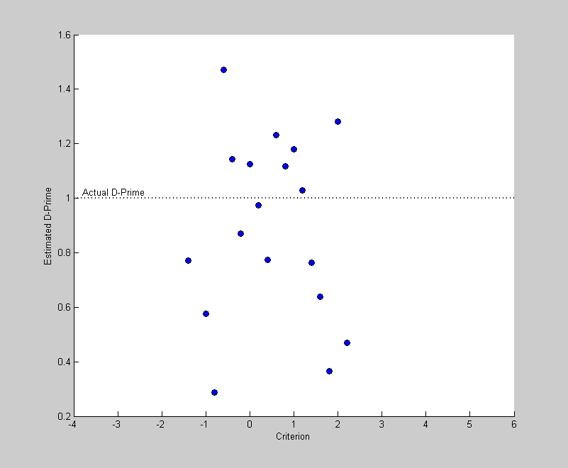
How accurate are our estimates of D-Prime? Not so good, really. In fact, for the criterion values near the high and low end of the range the values are not even plotted. What happened to those extreme values? Well, if the criterion is set too high, then you might not have any hits at all which makes the calculation of zHit impossible. Similarly, if the criterion is too low, then you may never make a correct rejection in 100 trials, which makes zCR invalid.

You may also notice that the valid estimates of D-Prime for extreme criterion values are particularly innacurate, and usually too low. This bias in these estimates of D-Prime means that we really can't just average across the D-Prime estimates. Instead, we'll perform an 'ROC' analysis on the data.

The ROC curve

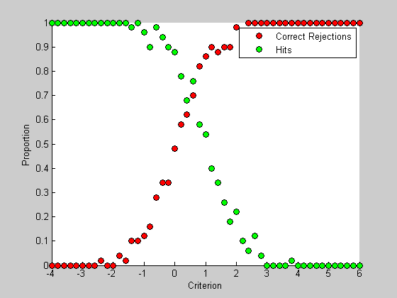
The hits and correct rejection rates vary hugely across the range of criterion values. As the criterion shifts from low to high, correct rejection rates go from 0 to 100% while hit rates go from 100% down to 0. Let's plot those values from our simulation

figure(2)
clf
hold on
h1= plot(criterionList,pCR,'ko','MarkerFaceColor','r');
h2= plot(criterionList,pHit,'ko','MarkerFaceColor','g');
legend([h1,h2],{'Correct Rejections','Hits'});
xlabel('Criterion');
ylabel('Proportion');

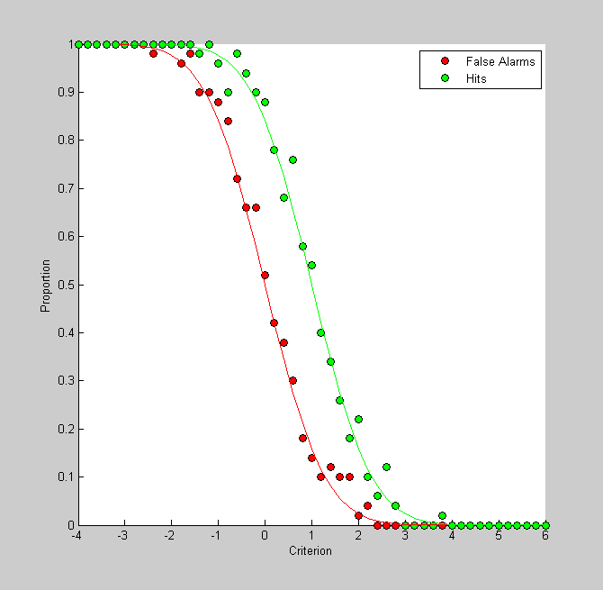
It's interesting to plot this graph with 'false alarms' instead of correct rejections. The proportion of false alarms is simply 1 minus the correct rejection rate:

pFA = 1-pCR;

figure(3)
clf
hold on
h1= plot(criterionList,pFA,'ko','MarkerFaceColor','r');
h2= plot(criterionList,pHit,'ko','MarkerFaceColor','g');
legend({'False Alarms','Hits'});
xlabel('Criterion');
ylabel('Proportion');

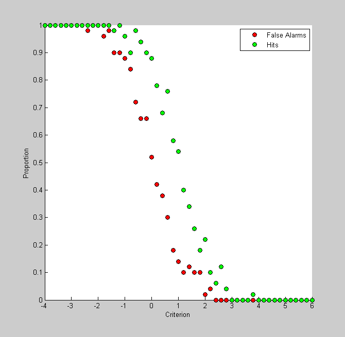
If this looks like two similarly-shaped curves shifted horizontally from eachother its because that's what they are. Remember, for a given criterion, pHit is the area to the curve under the signal distribution to the right. This is just 1 minus the cumulative distribution of the signal. Similarly, pFA is the area to the right of the criterion under the noise distribution - or 1 minus the cumulative distribution of the noise. Since the signal and noise distributions are defined as normal distribution with shifted means, this figure simply reflects the two cumulative normals, shifted by their means. The shift should be D-Prime.

The PsychToolbox comes with a cumulative normal function ('NormalCumulative') so we and use this to draw the 'actual' rates of hits and false alarms on the same graph:

pHitReal = 1-NormalCumulative(criterionList,signalMean,variance);
pFAReal = 1-NormalCumulative(criterionList,noiseMean,variance);

plot(criterionList,pFAReal,'r-');
plot(criterionList,pHitReal,'g-');

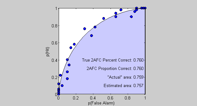
Another way of showing the relationship between hits and false alarms is to plot one against the other. This is the ROC curve, which is the proportion of hits plotted on the y-axis against false-alarms are on the x-axis.

figure(4)
clf

plot(pFA,pHit,'ko','MarkerFaceColor','b');
set(gca,'XLim',[0,1]);
set(gca,'YLim',[0,1]);
axis square
xlabel('p(False Alarm)');
ylabel('p(Hit)');

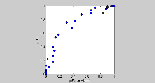
Each data point is the result of the simulation for each criterion value. Low criteria lead to points up in the upper-right corner and high-criterion values lead to points in the lower-left. Right? A low criterion value means the subject will almost always say 'yes', leading to nearly all trials being either false alarms or hits - the upper right corner.

What does this curve tell us about the strength of the signal (or D-Prime)? Looking at the previous figure you can see that if D-Prime was equal to zero, then the two curves would sit right on top of each other. The ROC curve would then be a series of points along y=x. On the other hand, if D-Prime is large enough that the signal and noise distributions don't overlap, then the false alarm rate would drop to zero before the hits would begin to fall below 1. The resulting ROC curve would therefore trace along the top of the graph until it hits the upper left corner, and then drop straight down.

ROC curves for values of D-Prime between these extremes look like the demonstration here - they bow out away from y=x. The amount of bowing is related to the size of D-Prime.

Using our evaluations of the cumulative normal above, We can show the 'real' ROC curve as a transparent 'patch' on the same graph:

patch([pFAReal,1],[pHitReal,0],'b','FaceAlpha',.2);

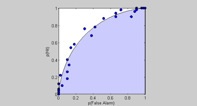
How well does the simlation match the expected ROC curve? You might notice that the simulated data 'looks' better plotted this way than it did when we plotted the estimated D-Prime values. This is because the wild estimates of D-Prime for extreme criterion values correspond to false alarm rates and hit rates that are compressed near 0 and 1 respectively.

Area under the ROC curve

A natural way to quantify the amount of 'bowing' in the ROC curve is to calculate the area under the curve. For a real (or simulated) data set, this involves 'numerical integration', which is basically adding up the areas of the rectangles (technically trapezoids) under the curve.

Matlab has a nice function for this called 'trapz' which performs numerical integration using the 'trapezoid rule' and allows for unequal (and even nonmonotonic) spacing for the sampling along the x-axis - exactly what we have here. The only weird thing is that our x-axis values (the false alarms) generally go from right to left, so 'trapz' gives us a negative number. So we'll just flip the sign.

% Area under the ROC curve based on the simulated data
AEst = -trapz(pFA,pHit)
% Area under the ROC curve based on the expected values
AReal = -trapz(pFAReal,pHitReal);

% Display the results as text in the figure
text(1,.1,sprintf('Estimated area: %5.3f ',AEst),'HorizontalAlignment','Right');
text(1,.2,sprintf('"Actual" area: %5.3f ',AReal),'HorizontalAlignment','Right');

AEst =

    0.7570

You can see how the estimated area is pretty close to the actual area, which means that this method of calculating the area under the ROC curve is a pretty good way of estimating the size of the difference between signal and noise - especially compared to taking the mean across the estiamtes of D-Prime as we discussed near the beginning of the lesson.

But what does this area mean? We discussed earlier that the bowing of the ROC curve increases with D-Prime. Quantitatively, this means that the area under the ROC curve ranges from a low value of 0.5 for D-Prime =0 (the area of the lower-right triangle) to a maximum value of 1.0 (the area of the whole square). Hmmm. 0.5 to 1.0. This sounds like a range of probabilities. In fact, we'll see in a moment that this exactly what this is.

Simulating a 2AFC trial:

While the yes/no experiment may be the simplest experiment you can run, you can see that a problem with it is that there is the free-parameter of the criterion value. If a subject chooses an extreme criterion value, the estimate of D-Prime will be innacurate. Even worse, if the criterion drifts within a block of trials then we're really in trouble. Also, calculating the whole ROC curve isn't easy because manipulating the criterion isn't trivial. The simulation we just ran involved 100 trials for each of 51 criterion - 5100 trials! That's clearly not efficient.

Fortunately psychophysicists have come up with the 2AFC method that is 'criterion free'. Recall in the motion coherence experiment we ran earlier that your choice on a given trial was based on which direction you thought the motion was going, not whether or not there was motion. You're forced to decide between two equally probable options and criterion plays no role.

In a traditional 2AFC experiment, subjects are shown a signal stimulus and a noise stimulus and are forced to choose which one had the signal. These stimuli can be presented in temporal succession, called 'two interval forced-choice' or next to eachother in space 'two alternative spatial forced choice'.

How do we predict a subject's decision in a 2AFC trial based on Signal Detection Theory? The idea is that the subject receives two internal responses in a given trial, one from the signal and one from the noise. The optimal decision rule is to decide that the signal belonged to the trial that produced the greatest internal response.

We can simulate the performance on a series of 2AFC trials really easily in Matlab. We'll use the same SDT probability distribution parameters that are left over from the simulations of the yes/no experiment.

% Generate vectors of internal responses for the signal and noise, one
% value for each trial.
internalRespSignal= randn(1,nTrials)*sqrt(variance)+signalMean;
internalRespNoise= randn(1,nTrials)*sqrt(variance)+noiseMean;

Correct decisions are made when internalRespSignal > internalRespNoise. Percent correct is calculated by adding up the number of trials where this happens and divide by nTrials:

pCorrect = sum(internalRespSignal>internalRespNoise)/nTrials;
% Display this number in the ROC graph
text(1,.3,sprintf('2AFC Proportion Correct: %5.3f ',pCorrect),'HorizontalAlignment','Right');

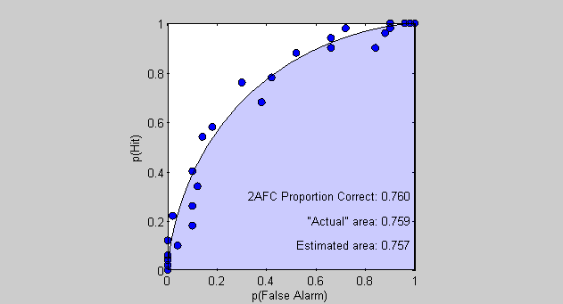
Look at that! The estimated percent correct is very close to the area under the ROC curve. In the limit this is a true fact. The area under the ROC curve is equal to the performance expected in a 2AFC task.

The calculus behind why this is true isn't too complicated but it's beyond the scope of this Matlab lesson. Check out Green and Swet's (1966) book if you're interested.

% Finally, there is a simple way to estimate D-prime from this probability,
% which is by converting the percent correct (or area under the curve) to a
% z-score using the inverse of the normal CDF, and multiplying by square
% root of two:

%From the 2AFC simulation:
EstDPrime2AFC = sqrt(2)*inverseNormalCDF(pCorrect)

%From the estimated area under the curve:
EstDPrimeAEst = sqrt(2)*inverseNormalCDF(AEst)

%From the "actual" area under the curve:
EstDPrimeAReal = sqrt(2)*inverseNormalCDF(AReal)

EstDPrime2AFC =

    0.9989


EstDPrimeAEst =

    0.9853


EstDPrimeAReal =

    0.9965

%All are pretty close to 1.  Of course, we can go the other way around and
%calculate what the performance on the 2AFC task should be in the limit -
%and also the true area under the ROC using the normal cumulative
%distribution function:

limitPCorrect = NormalCumulative(dPrime/sqrt(2),0,1);
text(1,.4,sprintf('True 2AFC Percent Correct: %5.3f ',limitPCorrect),'HorizontalAlignment','Right');

Differences between the 'limitPCorrect' and the 'actual' area under the curve is the result of our finite sampling of the criterion values and the numerical estimation of the area under the curve. 'limitPCorrect' is the most accurate estimate of the expected percent correct and the area under the curve.

Generating a psychometric function with the ideal observer

It should now be clear how easy it is to simulate a response to a 2AFC trial using SDT. We can now vary the stimulus strength to build a psychometric function and fit a Weibull to the results to estimate a threshold. This is a useful exercise for testing how well your choice of experimental parameters will lead to a reliable estimate of the threshold. You can also use simulations like this to see how robust your estimates are to things like key-press errors.

To start with, we need to make up a relation between the physical stimulus strength (e.g. coherence) and the corresponding mean of the signal used for SDT. Coherence ranges between 0 (hard) and 1 (very easy), so we can make D-Prime be the following function of coherence:

signalMean = k*inverseNormalCDF((coherence+1)/2)

Where k is a constant that we can vary. This is an arbitrary function - the real relation between the physical stimulus intensity and the expected internal response is an empirical question. How would you use psychophysics to measure it?

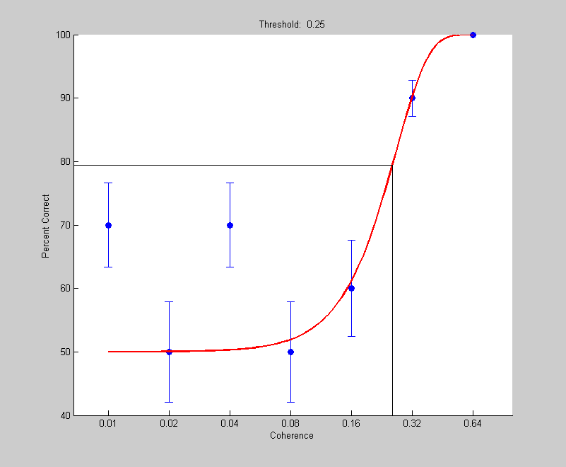
The next set of code will generate a 'results' structure based on the method of constant stimuli and an 'ideal observer' based on SDT:

k=5;

coherences = [.01,.02,.04,.08,.16,.32,.64];
nReps = 10;  %repetitions per coherence
nTrials = length(coherences)*nReps;
noiseMean = 0;
variance = 1;

coherenceList = repmat(coherences,nReps,1);

signalMean = k*inverseNormalCDF((coherenceList(:)'+1)/2);

results.intensity =coherenceList(:)';

internalRespSignal= randn(1,nTrials)*sqrt(variance)+signalMean;
internalRespNoise= randn(1,nTrials)*sqrt(variance)+noiseMean;
results.response  = internalRespSignal>internalRespNoise;

pInit.t = .1;
pInit.b = 3;
pInit.shutup = 1;

pBest = fit('fitPsychometricFunction',pInit,{'t','b'},results,'Weibull');
figure(1)
plotPsycho(results,'coherence',pBest,'Weibull');

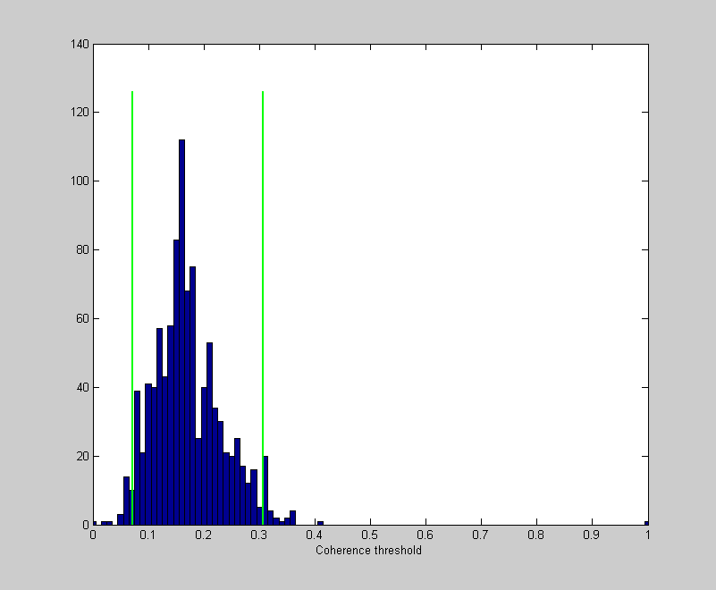
To evaluate how accurately we're estimating the threshold we can simulate 1000 'experiments'

pInit.t = .1;
pInit.b = 3;
pInit.shutup = 1;

tic
nExperiments = 1000;
thresh = zeros(1,nExperiments);
h = waitbar(0,sprintf('Running  %d experiments',nExperiments));
for i=1:nExperiments
    internalRespSignal= randn(1,nTrials)*sqrt(variance)+signalMean;
    internalRespNoise= randn(1,nTrials)*sqrt(variance)+noiseMean;
    results.response  = internalRespSignal>internalRespNoise;
    pBest = fit('fitPsychometricFunction',pInit,{'t','b'},results,'Weibull');
    thresh(i) = pBest.t;
    waitbar(i/nExperiments,h)
end
toc
delete(h);

Elapsed time is 446.564179 seconds.

Like we did for bootstrapping, we'll look at the histogram and calculate the middle 68% as our estimate of the standard error.

figure(1)
clf
hist(thresh,0:.01:1);
set(gca,'XLim',[0,1]);
hold on

CIrange = 95;
CI = [prctile(thresh,(100-CIrange)/2),prctile(thresh,(100+CIrange)/2)];
ylim = get(gca,'YLim');
plot(CI(1)*[1,1],ylim*1.05,'g-','LineWidth',2)
plot(CI(2)*[1,1],ylim*1.05,'g-','LineWidth',2)
xlabel('Coherence threshold');

What's the ideal observer's 'true' threshold? Remember that our threshold is defined to be the stimulus intensity that produces a percent correct of (1/2)^(1/3) - which is about 79%. We know that this corresponds to a D-Prime of:

dprimeThresh = inverseNormalCDF( (1/2)^(1/3))

% We defined the relation between the stimulus intensity and the signal
% mean to be k*inverseNormalCDF((cThresh+1)/2), so D-Prime will be
% k*inverseNormalCDF((cThresh+1)/2)/sqrt(variance).  Doing some algebra and
% solving for c gives:

cThresh = 2*NormalCumulative(sqrt(2*variance)*dprimeThresh/k,0,1)-1

nTrials = 10000;

signalMean = k*inverseNormalCDF((cThresh+1)/2);

internalRespSignal= randn(1,nTrials)*sqrt(variance)+signalMean;
internalRespNoise= randn(1,nTrials)*sqrt(variance)+noiseMean;
results.response  = internalRespSignal>internalRespNoise;
pc = sum(results.response)/nTrials;
disp(sprintf('Percent correct intensity of %5.3g after %d trials: %5.3g: Expected: %5.3g',...
    cThresh,nTrials,pc,(1/2)^(1/3)));

dprimeThresh =

    0.8193


cThresh =

    0.1833

Percent correct intensity of 0.183 after 10000 trials: 0.794: Expected: 0.794

Summary

In summary, we showed that a simulated experiment of a standard yes/no experiment can lead to variable estimates of D-Prime depending on the criterion. The ROC curve, which plots hits against false alarm rates provides a nice summary of the results of the simulation for the range of criterion values. We showed that the area under the ROC curve is the same value as the percent correct you'd get in a 2AFC experiment using the same stimuli. Finally, we can convert from this percent correct (or area under the curve) to D-Prime using the inverse of the normal CDF which provides a reliable way to estimate D-Prime from the yes/no experiments.

Exercises

Published with MATLAB® 7.6